Properties of Fluids#
Understanding the physical properties of fluids is essential for analyzing fluid flow. The key properties include:
Density (\(\rho\))
Specific Weight (\(\gamma\))
Specific Gravity (\(SG\))
Viscosity (\(\mu\))
Surface Tension (\(\sigma\))
What is Density?#
Density is a fundamental property of fluids that measures the amount of mass contained in a unit volume of a substance. It is a key parameter in fluid mechanics, as it influences various aspects of fluid behavior, including pressure, buoyancy, and flow dynamics. Density is denoted by the symbol \(\rho\) and is mathematically expressed as:
Where:
\(\rho\) is the density (in units of \(kg/m^3\) in SI),
\(m\) is the mass of the fluid (in kilograms, kg),
\(V\) is the volume of the fluid (in cubic meters, \(m^3\)).
Importance of Density in Fluid Mechanics#
Density plays a crucial role in several fluid mechanics applications:
Buoyancy: Objects float or sink in a fluid depending on their density relative to the fluid. For instance, a boat floats because its average density is less than the density of water.
Pressure in a Fluid Column: The pressure at a given depth in a fluid is directly proportional to its density (hydrostatic pressure equation: \(P = \rho gh\), where \(g\) is the acceleration due to gravity and \(h\) is the depth).
Flow Behavior: In compressible flows (e.g., gases), density changes significantly and must be accounted for. In incompressible flows (e.g., liquids), density is generally constant.
Note
In liquids, density variations are usually negligible except in thermal expansion problems.
In gases, density is a strong function of pressure and temperature, making it central to compressible flow analysis.
Examples of Density#
Water: The density of water at standard temperature and pressure (STP) is approximately \(1000 \, kg/m^3\). This property is commonly used as a reference for other fluids.
Air: The density of air at sea level and room temperature is about \(1.225 \, kg/m^3\). This value decreases with altitude.
Mercury: Mercury has a very high density of approximately \(13,600 \, kg/m^3\), which is why it is commonly used in barometers to measure atmospheric pressure.
Typical Densities of Fluids#
The following table lists the typical densities of common fluids in both SI units and British Gravitational (BG) units.
Fluid |
Density (\(kg/m^3\)) |
Density (\(lb/ft^3\)) |
Remarks |
|---|---|---|---|
Air (STP) |
1.225 |
0.0765 |
At sea level |
Water (STP) |
1000 |
62.4 |
Standard temperature |
Seawater |
1025 |
64 |
Higher than fresh water due to salts |
Mercury |
13,600 |
847 |
Extremely dense liquid |
Ethanol |
789 |
49.3 |
Common alcohol |
Glycerin |
1260 |
78.6 |
Viscous liquid |
Gasoline |
680 |
42.5 |
Common fuel |
Units of Density#
SI Units: In the International System of Units (SI), density is measured in kilograms per cubic meter (\(kg/m^3\)). This unit reflects the mass contained in one cubic meter of a substance.
BG Units: In the British Gravitational (BG) system, density is measured in pounds per cubic foot (\(lb/ft^3\)), which represents the weight of the fluid per unit volume in cubic feet.
Practical Example: Buoyancy#
Consider an object submerged in water. If the object’s density is less than that of water (\(\rho_{\text{object}} < \rho_{\text{water}}\)), it will float. For example, a wooden block with a density of \(600 \, kg/m^3\) will float in water because its density is significantly lower than water’s density of \(1000 \, kg/m^3\).
On the other hand, if an object is denser than water (e.g., iron with \(\rho \approx 7,870 \, kg/m^3\)), it will sink because its density is much greater than the surrounding fluid.
What is Specific Weight?#
Specific weight (also known as weight density) is the weight of a fluid per unit volume. It is a measure of how much weight is associated with a given volume of the substance. Specific weight is denoted by the symbol \(\gamma\) and is related to the density of the fluid.
Mathematically, specific weight is expressed as:
Where:
\(\gamma\) is the specific weight (in units of \(N/m^3\) or \(lbf/ft^3\)),
\(\rho\) is the density of the fluid (in units of \(kg/m^3\) or \(slug/ft^3\)),
\(g\) is the gravitational acceleration (standard value \(9.81 \, m/s^2\) or \(32.174 \, ft/s^2\)).
Units of Specific Weight#
SI Units: In the SI system, specific weight is measured in newtons per cubic meter (\(N/m^3\)), which represents the weight (force) in newtons of a fluid in one cubic meter of volume.
\[ \gamma \ (\text{SI units}) = \rho \times 9.81 \, m/s^2 \]Imperial/US Units: In the Imperial system, specific weight is commonly measured in pounds-force per cubic foot (\(lbf/ft^3\)).
\[ \gamma \ (\text{Imperial units}) = \rho \times 32.174 \, ft/s^2 \]
Relationship Between Density and Specific Weight#
The specific weight is directly proportional to the density of the fluid. For a fluid with constant density, the specific weight is simply the density multiplied by the acceleration due to gravity. If a fluid’s density changes with temperature or pressure, its specific weight will also change.
Example: Specific Weight of Water#
In SI Units: The density of water at \(4^\circ C\) is approximately \(1000 \, kg/m^3\). Using the acceleration due to gravity \(g = 9.81 \, m/s^2\), the specific weight of water is:
\[ \gamma_{\text{water}} = 1000 \, \text{kg/m}^3 \times 9.81 \, \text{m/s}^2 = 9810 \, \text{N/m}^3 \]In the BG System: The density of water in the BG system is approximately \(1.94 \, \text{slug/ft}^3\). Using \(g = 32.174 \, \text{ft/s}^2\), the specific weight of water is:
\[ \gamma_{\text{water}} = 1.94 \, \text{slug/ft}^3 \times 32.174 \, \text{ft/s}^2 = 62.4 \, \text{lbf/ft}^3 \]
In the BG system, the specific weight of water remains 62.4 lbf/ft³, as it accounts for both the density in slugs and the gravitational acceleration.
Practical Applications of Specific Weight#
Specific weight is often used in calculations involving:
Buoyancy: The weight of the displaced fluid determines the buoyant force on an object.
Hydrostatics: The pressure exerted by a fluid at rest depends on the specific weight, as seen in the hydrostatic pressure formulation \(P = \gamma h\), where \(h\) is the height of the fluid column.
Hydraulic Systems: Engineers use specific weight to design systems where fluid flow and pressures are key factors, such as in dams or water distribution systems.
Table of Specific Weights for Common Fluids#
Fluid |
Density (\(\rho\)) |
Specific Weight (\(\gamma\)) in SI |
Specific Weight (\(\gamma\)) in BG Units |
|---|---|---|---|
Air (STP) |
1.225 kg/m³ |
12.01 N/m³ |
0.0765 lbf/ft³ |
Water (4°C) |
1000 kg/m³ |
9810 N/m³ |
62.4 lbf/ft³ |
Seawater |
1025 kg/m³ |
10,055 N/m³ |
64.0 lbf/ft³ |
Mercury |
13,600 kg/m³ |
133,416 N/m³ |
847 lbf/ft³ |
Ethanol |
789 kg/m³ |
7744.1 N/m³ |
49.3 lbf/ft³ |
Glycerin |
1260 kg/m³ |
12,355 N/m³ |
78.6 lbf/ft³ |
Summary#
Specific weight is the weight per unit volume of a substance and is given by the product of density and gravitational acceleration.
It is widely used in fluid mechanics to calculate pressures, buoyancy forces, and other parameters related to the weight of fluids.
Specific weight changes with variations in density and is influenced by temperature, pressure, and fluid composition.
Understanding the specific weight is crucial in applications such as hydrostatics, hydraulics, and fluid dynamics.
What is Specific Gravity?#
Specific gravity (denoted as \(SG\)) is the ratio of the density of a substance to the density of a reference substance, usually water for liquids and solids, or air for gases. Since it is a ratio of two densities, specific gravity is a dimensionless quantity.
For liquids and solids, the reference substance is water at \(4^\circ C\), which has a density of approximately \(1000 \, \text{kg/m}^3\) in the SI system or \(62.4 \, \text{lb/ft}^3\) in the English system.
where:
\(\rho_{\text{fluid}}\) is the density of the fluid (or material) whose specific gravity is being calculated,
\(\rho_{\text{water}}\) is the density of water at \(4^\circ C\).
Since the densities are in the same units, the specific gravity itself has no units.
Example Calculation#
If the density of mercury is \(13,600 \, \text{kg/m}^3\), the specific gravity of mercury relative to water would be:
Interpretation#
A specific gravity greater than 1 means the substance is denser than water.
A specific gravity less than 1 means the substance is less dense than water.
For example, the specific gravity of ethanol is 0.789, meaning ethanol is less dense than water.
Applications#
Buoyancy: Specific gravity helps in determining whether an object will float or sink in a fluid.
Concentration: It is used to estimate concentrations in solutions, especially in industries like brewing and chemical processing.
Hydrometry: Devices like hydrometers use specific gravity to measure the density of liquids.
Table of Specific Gravities for Common Substances#
Substance |
Specific Gravity (Relative to Water) |
|---|---|
Water |
1.00 |
Mercury |
13.6 |
Ethanol |
0.789 |
Seawater |
1.025 |
Glycerin |
1.26 |
Air (Relative to Water) |
0.00123 |
Note that for gases, specific gravity is often measured relative to air rather than water.
Note
Archimedes — Father of Hydrostatics
Lifespan: 287–212 BCE, born in Syracuse, studied in Alexandria.
Major Contributions:
On Floating Bodies → Principle of buoyancy, density, specific gravity.
Lever law and simple machines → “Give me a place to stand, and I will move the world.”
Archimedean screw → Water lifting for irrigation.
Mathematical advances → Method of exhaustion (proto-calculus), close estimate of π.
Context:
Patronized by King Hiero II of Syracuse.
Possible student of Conon of Samos in Alexandria.
Killed during the Roman conquest, despite orders to spare him.
Allies:
Conon of Samos → mentor and friend in Alexandria.
Eratosthenes → correspondent, recipient of The Method.
Dositheus of Pelusium → disciple, to whom works were dedicated.
King Hiero II → political ally and patron.
Rivals & Tensions:
Apollonius of Perga → geometry vs. mechanics; no open feud, but intellectual contrast.
Romans → feared his war machines; ultimately his military “rivals.”
Critics in Alexandria → annoyed at his secrecy and challenges without proofs.
Quirks & Gossip:
“Eureka!” bath story (likely apocryphal but legendary).
Absorbed in diagrams — said to forget food, sleep, even war.
Built war machines but disliked being remembered for them.
Legacy:
True father of hydrostatics and one of the founding figures of mechanics.
His fusion of mathematics and mechanics paved the way for Galileo, Newton, and modern fluid dynamics.
Ideal Gas Law#
The Ideal Gas Law can also be expressed in terms of the specific form as:
where:
\(P\) is the pressure of the gas (in Pascals, Pa),
\(\rho\) is the density of the gas (in \(\text{kg/m}^3\)),
\(R\) is the specific gas constant (in J/kg·K),
\(T\) is the absolute temperature of the gas (in Kelvin, K).
Conceptualization#
This form of the Ideal Gas Law relates the pressure of a gas to its density rather than the amount of gas in moles (\(n\)). The specific gas constant \(R\) here is related to the universal gas constant \(R_u\) by:
where:
\(R_u = 8.314 \, \text{J/mol·K}\) is the universal gas constant,
\(M\) is the molar mass of the gas (in kg/mol).
For example, the specific gas constant \(R\) for dry air is approximately \(287 \, \text{J/kg·K}\).
Understanding the Equation#
The equation \(P = \rho R T\) shows that pressure is directly proportional to both the density of the gas and its temperature.
Higher density at a constant temperature results in higher pressure.
Similarly, increasing the temperature at a constant density will also increase the pressure.
This form is particularly useful in atmospheric science and fluid dynamics, where density \(\rho\) is often a more convenient quantity than the number of moles.
Relationship to the Molar Form#
The traditional molar form of the Ideal Gas Law is:
where:
\(P\) is the pressure,
\(V\) is the volume,
\(n\) is the number of moles,
\(R_u\) is the universal gas constant (\(8.314 \, \text{J/mol·K}\)),
\(T\) is the absolute temperature.
To derive \(P = \rho R T\), we start by expressing density \(\rho\) as the mass per unit volume:
Also, the number of moles \(n\) is related to the mass \(m\) and the molar mass \(M\) by:
Substituting \(n = \frac{m}{M}\) into the Ideal Gas Law:
Since \(\frac{m}{V} = \rho\), we now have:
Thus, the equation becomes:
where \(R = \frac{R_u}{M}\) is the specific gas constant for the particular gas being considered.
Summary#
\(R_u\) is the universal gas constant.
\(R = \frac{R_u}{M}\) is the specific gas constant, which depends on the molar mass of the gas.
Example Calculation#
Let’s calculate the pressure of dry air with a density of \(1.2 \, \text{kg/m}^3\) at a temperature of \(300 \, \text{K}\), using the specific gas constant \(R = 287 \, \text{J/kg·K}\) for air.
So, the pressure is approximately 103.3 kPa.
Applications of \(P = \rho R T\)#
This form of the Ideal Gas Law is often used in fields like:
Atmospheric science: to describe the behavior of gases in the atmosphere.
Fluid mechanics: especially when analyzing compressible flows.
Aerospace engineering: to model air properties in high-speed flight.
Assumptions of the Ideal Gas Law#
Like the molar form, this specific form of the Ideal Gas Law assumes:
No intermolecular forces: The gas molecules do not attract or repel each other.
Point particles: Gas molecules are considered to have negligible volume.
Elastic collisions: All collisions between gas molecules and with container walls are perfectly elastic.
Valid at low pressures and high temperatures: The law breaks down under extreme conditions (high pressure, low temperature).
Limitations#
The Ideal Gas Law, in this form, is an approximation that assumes ideal behavior. For real gases under conditions of high pressure or low temperature, deviations occur, and more complex equations, such as the Van der Waals equation, must be used.
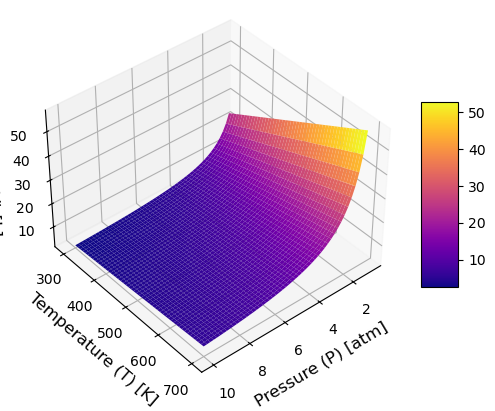
Python: Matplotlib Static#
import numpy as np
import matplotlib.pyplot as plt
from mpl_toolkits.mplot3d import Axes3D

# Create a figure
fig = plt.figure()
ax = fig.add_subplot(111, projection='3d')

# Define ranges for temperature (T) and pressure (P)
T = np.linspace(300, 700, 50)  # Temperature from 300K to 700K
P = np.linspace(1, 10, 50)     # Pressure from 1 to 10 atm
T, P = np.meshgrid(T, P)

# Equation for volume V, assume ideal gas law: PV = nRT
R = 0.0821  # L·atm/mol·K (Ideal gas constant)
n = 1       # Assume 1 mole of gas
V = (n * R * T) / P  # Ideal gas law rearranged to V = nRT / P

# Plot the surface in color
surf = ax.plot_surface(P, T, V, cmap='plasma', edgecolor='none')

# Color bar for the surface
fig.colorbar(surf, ax=ax, shrink=0.5, aspect=5)

# Label axes with units
ax.set_xlabel('Pressure (P) [atm]', fontsize=12)
ax.set_ylabel('Temperature (T) [K]', fontsize=12)
ax.set_zlabel('Volume (V) [L]', fontsize=12)

# Rotate the plot by 90 degrees
ax.view_init(elev=40, azim=50)  # azim=90 rotates it by 90 degrees

plt.show()
Python: Matplotlib Interactive I#
import numpy as np
import plotly.graph_objects as go
from plotly.offline import init_notebook_mode

# Initialize Plotly to work in notebook mode for Jupyter environments
init_notebook_mode(connected=True)

# Define ranges for temperature (T) and pressure (P)
T = np.linspace(300, 700, 50)  # Temperature from 300K to 700K
P = np.linspace(1, 10, 50)     # Pressure from 1 to 10 atm
T, P = np.meshgrid(T, P)

# Equation for volume V, using the ideal gas law: PV = nRT
R = 0.0821  # Ideal gas constant in L·atm/mol·K
n = 1       # Assume 1 mole of gas
V = (n * R * T) / P  # Rearranged ideal gas law to V = nRT / P

# Create an interactive 3D surface plot with Plotly
fig = go.Figure(data=[go.Surface(z=V, x=P, y=T, colorscale="Plasma")])

# Update layout for the plot
fig.update_layout(
    title="Ideal Gas Law: Volume as a Function of Pressure and Temperature",
    scene=dict(
        xaxis_title="Pressure (P) [atm]",
        yaxis_title="Temperature (T) [K]",
        zaxis_title="Volume (V) [L]",
        camera=dict(eye=dict(x=1.2, y=1.2, z=0.8))  # Set view angle
    ),
    coloraxis_colorbar=dict(
        title="Volume [L]",
        titleside="right"
    )
)

# Show plot
fig.show()
Python: Plotly Interactive II#
import numpy as np
import plotly.graph_objects as go

# Define ranges for temperature (T) and pressure (P)
T = np.linspace(300, 700, 50)  # Temperature from 300K to 700K
P = np.linspace(1, 10, 50)     # Pressure from 1 to 10 atm
T, P = np.meshgrid(T, P)

# Equation for volume V, using the ideal gas law: PV = nRT
R = 0.0821  # Ideal gas constant in L·atm/mol·K
n = 1       # Assume 1 mole of gas
V = (n * R * T) / P  # Rearranged ideal gas law to V = nRT / P

# Create 3D surface plot
fig = go.Figure()

# Add 3D surface with reduced opacity
fig.add_trace(go.Surface(z=V, x=P, y=T, colorscale="Plasma", opacity=0.5))

# Interactive cross-sections for projections
def add_projection(fig, P_val=None, T_val=None, V_val=None):
    if P_val:
        # Slice at a specific Pressure (P) value
        V_slice = (n * R * T) / P_val
        fig.add_trace(go.Scatter3d(
            x=np.full(T.shape[0], P_val), y=T[:,0], z=V_slice[:,0],
            mode="lines", line=dict(color="blue", width=6),
            name=f"Projection at P={P_val} atm"))
    if T_val:
        # Slice at a specific Temperature (T) value
        V_slice = (n * R * T_val) / P
        fig.add_trace(go.Scatter3d(
            x=P[0], y=np.full(P.shape[1], T_val), z=V_slice[0],
            mode="lines", line=dict(color="green", width=6),
            name=f"Projection at T={T_val} K"))
    if V_val:
        # Slice at a specific Volume (V) value
        P_slice = (n * R * T) / V_val
        fig.add_trace(go.Scatter3d(
            x=P_slice[0], y=T[:,0], z=np.full(T.shape[0], V_val),
            mode="lines", line=dict(color="red", width=6),
            name=f"Projection at V={V_val} L"))

# Initial projections
add_projection(fig, P_val=5)
add_projection(fig, T_val=500)
add_projection(fig, V_val=20)

# Update layout
fig.update_layout(
    title="Ideal Gas Law with Enhanced 2D Projections",
    scene=dict(
        xaxis_title="Pressure (P) [atm]",
        yaxis_title="Temperature (T) [K]",
        zaxis_title="Volume (V) [L]",
        camera=dict(eye=dict(x=1.2, y=1.2, z=0.8))  # Set view angle
    ),
    coloraxis_colorbar=dict(
        title="Volume [L]",
        titleside="right"
    )
)

fig.show()
Viscosity: Description and Derivation#
Introduction to Viscosity#
Viscosity is a measure of a fluid’s resistance to deformation under shear stress. In simple terms, it quantifies how “thick” or “sticky” a fluid is. High-viscosity fluids like honey resist flow more than low-viscosity fluids like water. Viscosity plays a critical role in fluid mechanics, affecting flow behavior in various applications ranging from lubrication to aerodynamics.
Viscosity arises from the internal friction between layers of fluid in motion. When fluid moves, the layers adjacent to solid boundaries experience resistance due to intermolecular forces, and this interaction causes the “stickiness” that characterizes viscous effects.
In fluids, viscosity depends on:
Temperature: Higher temperatures generally decrease the viscosity of liquids and increase the viscosity of gases.
Pressure: For most liquids, the viscosity slightly increases with pressure, while for gases, this effect is more complex.
The no-slip condition is a fundamental boundary condition in fluid mechanics, particularly relevant in the context of viscosity. It states that at a solid boundary, a fluid will have zero velocity relative to the boundary. In other words, the fluid particles at the interface between the fluid and the solid surface “stick” to the surface, meaning that the velocity of the fluid at the boundary is equal to the velocity of the surface itself.
Role of the No-Slip Condition in Viscous Flows#
Viscosity, as described earlier, is a measure of a fluid’s internal resistance to deformation or shear. When fluid flows over a surface, such as a pipe wall or a flat plate, the no-slip condition creates a velocity gradient from zero at the boundary (due to the fluid adhering to the surface) to the maximum velocity in the flow field away from the surface. This velocity gradient generates shear stress in the fluid, with the magnitude of this stress being directly proportional to the viscosity of the fluid.
For a highly viscous fluid, such as honey, the velocity gradient near the surface is more gradual, meaning the fluid’s motion near the boundary is significantly slowed down by viscous forces. In contrast, for low-viscosity fluids like water, the fluid velocity increases more sharply away from the surface, as the internal friction is lower.
Physical Mechanism Behind the No-Slip Condition#
The no-slip condition arises due to intermolecular forces between the fluid molecules and the solid boundary. Near the surface, fluid molecules are attracted to the solid and do not slip past it. The layer of fluid molecules closest to the surface is essentially stationary relative to the solid. The fluid layers adjacent to this stationary layer experience shear due to the velocity difference between layers, and this is where viscosity acts to resist the relative motion between the layers.
In summary:
Viscosity: Determines how much the fluid resists the development of this velocity gradient.
No-slip condition: Ensures that the velocity of the fluid at the boundary equals the velocity of the solid surface, enforcing a zero-velocity condition at solid-fluid interfaces.
Importance in Applications#
The no-slip condition is critical in various engineering applications where fluid interaction with solid surfaces is important:
Lubrication: In systems where moving parts are lubricated, the no-slip condition ensures a velocity gradient develops in the lubricant, creating shear stress that supports the load.
Aerodynamics: In aerodynamics, the no-slip condition causes the formation of boundary layers on surfaces like airplane wings, which significantly affect drag and lift.
Heat transfer: In heat exchangers, the no-slip condition at the solid walls enhances heat transfer by enforcing fluid velocity gradients, which increase convective heat transfer.
Thus, the no-slip condition is inseparably linked with viscosity, as it governs the behavior of fluids at solid boundaries, directly influencing the velocity distribution and the shear forces in the fluid.
Shear Flow in Fluids#
Consider a Newtonian fluid between two parallel plates, where:
The bottom plate is stationary.
The top plate moves at a constant velocity \(U\).
The fluid between the plates is assumed to be incompressible and Newtonian.
The distance between the plates is \(h\).
The velocity distribution between the plates is linear, given by:
where \(u(y)\) is the fluid velocity at a distance \(y\) from the stationary plate.
The viscosity \(\mu\) is defined for Newtonian fluids (those for which the stress is proportional to the rate of strain) as the constant of proportionality between the shear stress \(\tau\) and the velocity gradient \(\frac{du}{dy}\) in a simple shear flow:
For Newtonian fluids, \(\mu\) remains constant, meaning the fluid’s resistance to shear flow is directly proportional to the velocity gradient. Non-Newtonian fluids, by contrast, exhibit a non-linear relationship between shear stress and velocity gradient, where viscosity may vary with the rate of strain.
For this system:
Thus, the shear stress is:
This shows that the shear stress \(\tau\) is directly proportional to the viscosity \(\mu\) and the velocity gradient \(\frac{U}{h}\).
Note
Remember:
\(\tau\) is the shear stress (force per unit area) acting parallel to the fluid layer,
\(\frac{du}{dy}\) is the velocity gradient (rate of strain) perpendicular to the fluid motion,
\(\mu\) is the dynamic viscosity (units: \(\text{Pa} \cdot \text{s}\) or \(\text{N} \cdot \text{s}/\text{m}^2\)).
In SI: \(\text{Pa} \cdot \text{s}\) or \(\text{N} \cdot \text{s}/\text{m}^2\).
In the CGS system: Poise (P), where \(1 \, \text{P} = 0.1 \, \text{Pa} \cdot \text{s}\).
Another common term is kinematic viscosity \(\nu\), defined as the ratio of dynamic viscosity to fluid density \(\rho\):
The units of kinematic viscosity are \(\text{m}^2/\text{s}\) (SI) and Stokes (St) in the CGS system.
Microscopic Origin of Viscosity#
From a molecular perspective, viscosity is related to the momentum transfer between fluid molecules. In gases, molecules move randomly, and as they collide, they transfer momentum, creating a shear stress. In liquids, the intermolecular forces dominate, and these forces resist the relative motion of adjacent layers, contributing to the fluid’s viscosity.
Experimental Measurement of Viscosity#
Viscosity can be measured using several devices, such as:
Capillary Viscometers: Based on measuring the flow rate of the fluid through a thin tube.
Rotational Viscometers: Measure the torque required to rotate a disk or cylinder in the fluid.
Falling Sphere Viscometers: Measure the terminal velocity of a sphere falling through the fluid, applying Stokes’ law.
Importance of Viscosity in Fluid Mechanics#
Viscosity is a fundamental property that governs how fluids resist motion under applied forces. It is particularly important in understanding fluid flow in systems ranging from simple pipe flows to complex aerodynamic applications. Newton’s law of viscosity provides the foundation for analyzing fluid behavior in shear flows, allowing us to predict stresses, velocities, and flow rates in Newtonian fluids. Derived from Newton’s law of viscosity, this property governs many fluid behaviors in both laminar and turbulent regimes.
In real-world engineering applications, accurate knowledge of viscosity is essential for designing fluid systems, analyzing heat transfer, and ensuring the efficient operation of machinery.
Laminar vs. Turbulent Flow: High viscosity favors laminar flow, while low viscosity fluids are more prone to turbulence.
Boundary Layers: Viscosity plays a critical role in the formation and thickness of boundary layers.
Energy Dissipation: Viscous effects lead to energy dissipation in fluids, important in pipe flow, pumps, and engines.
Surface Tension in Fluid Mechanics#
Surface Tension is a phenomenon where the surface of a liquid behaves like a stretched elastic membrane due to intermolecular forces. At a molecular level, this effect arises because molecules at the liquid’s surface experience a net inward force from neighboring molecules in the liquid, while molecules in the bulk experience balanced forces in all directions. This imbalance creates a “tension” on the surface, making it behave as if covered by an elastic film.
Importance and Applications#
Surface tension has significant effects in both natural and engineering systems:
Capillary Action: Surface tension enables liquids to flow in narrow spaces without external forces. For example, water can rise in thin tubes (capillaries), essential in biological processes like water transport in plants.
Droplet Formation: Surface tension is responsible for the spherical shape of liquid droplets. This is crucial in applications like inkjet printing and fuel injection systems, where controlled droplet formation is essential for proper functioning.
Soap Bubbles: Surface tension allows the formation of thin films that can enclose air, creating bubbles. Surfactants (like soap) reduce surface tension, stabilizing the film, which is why soap bubbles are so commonly observed.
Small-Scale Systems: In microfluidics and biomedical devices, surface tension forces dominate over gravitational forces due to the small scale. Engineers use this property to manipulate small fluid volumes precisely.
Practical Example: Maximum Internal Pressure in a Soap Bubble#
A classic problem in surface tension analysis involves determining the maximum internal pressure within a soap bubble.
When a soap bubble forms, it has two surfaces (inside and outside) exposed to air. The surface tension (\( \sigma \)) generates a pressure difference (\( \Delta P \)) across these surfaces.
For a soap bubble with radius \( r \), the pressure difference across the bubble’s surface can be derived using the Young-Laplace equation:
This equation accounts for the fact that a soap bubble has two layers (inner and outer surfaces), each contributing to the surface tension.
Example Calculation#
Let’s determine the maximum internal pressure of a soap bubble with a radius of \( r = 0.01 \, \text{m} \) and a surface tension of \( \sigma = 0.03 \, \text{N/m} \).
Given Data:
Radius, \( r = 0.01\), \(\text{m} \)
Surface tension, \( \sigma = 0.03 \), \(\text{N/m} \)
Applying the Formula:
\[ \Delta P = \frac{4 \sigma}{r} \]Substitute the Values:
\[ \Delta P = \frac{4 \times 0.03}{0.01} = \frac{0.12}{0.01} = 12 \, \text{Pa} \]
So, the maximum internal pressure of the soap bubble is \( 12 \), \(\text{Pa} \) greater than the external atmospheric pressure.
Summary#
Surface tension is a vital phenomenon that significantly affects fluid behavior in various contexts. Understanding and applying principles of surface tension, like in the above calculation, is essential in designing and analyzing systems in fields as diverse as biomedicine, environmental science, and engineering.
Interactive Python Exercise: Surface Tension and Droplet Shape#
This interactive exercise uses Python and Plotly to simulate how surface tension affects the shape of a droplet. We’ll create a plot that demonstrates how the pressure difference needed to maintain a certain droplet size changes with surface tension.
The Young-Laplace equation for a droplet on a surface is:
Where:
\( \Delta P \) is the pressure difference,
\( \sigma \) is the surface tension, and
\( r \) is the radius of the droplet.
The user can adjust the surface tension and observe its effect on the pressure difference and, consequently, the curvature of the droplet.
Code#
Below is the Python code. The exercise allows you to adjust the surface tension value and see the corresponding pressure difference required to maintain the droplet’s shape.
import numpy as np
import plotly.graph_objects as go
from ipywidgets import interact, FloatSlider

# Constants
r = 0.01  # Fixed radius of the droplet in meters

# Function to calculate pressure difference based on surface tension
def surface_tension_plot(sigma):
    # Calculate pressure difference
    delta_p = 2 * sigma / r

    # Set up data for the droplet shape (a semi-circle profile view)
    theta = np.linspace(0, np.pi, 100)  # Angle for the semi-circle
    x = r * np.cos(theta)  # x-coordinates for the droplet's surface
    y = r * np.sin(theta)  # y-coordinates for the droplet's surface

    # Plotting the droplet and the pressure difference
    fig = go.Figure()

    # Droplet shape (semi-circle)
    fig.add_trace(go.Scatter(x=x, y=y, mode='lines', name='Droplet Surface',
                             line=dict(color='blue', width=3)))

    # Show the pressure difference as text
    fig.add_annotation(x=0, y=0.015,
                       text=f"Pressure Difference (ΔP): {delta_p:.2f} Pa",
                       showarrow=False,
                       font=dict(size=14),
                       align="center")

    # Layout settings
    fig.update_layout(
        title=f"Droplet Shape with Surface Tension σ = {sigma:.2f} N/m",
        xaxis_title="x [m]",
        yaxis_title="y [m]",
        xaxis=dict(scaleanchor="y", scaleratio=1),
        yaxis=dict(range=[0, 0.02]),
        showlegend=False
    )

    fig.show()

# Interactive slider for surface tension
interact(surface_tension_plot, sigma=FloatSlider(value=0.03, min=0.01, max=0.1, step=0.01, description="Surface Tension (σ)"));
Explanation of the Surface Tension Interactive Exercise#
The following code demonstrates how surface tension affects the pressure difference needed to maintain a droplet’s curvature. By using the Young-Laplace equation, we can explore how varying the surface tension changes this pressure difference.
Young-Laplace Equation for a Droplet#
The Young-Laplace equation describes the relationship between surface tension and pressure difference for a droplet:
Where:
\(\Delta P\) is the pressure difference across the droplet’s surface,
\(\sigma\) is the surface tension (adjustable with a slider in the interactive example),
\(r\) is the radius of the droplet.
In this exercise, the radius \(r\) is held constant at \(0.01\), \(\text{m}\), allowing us to see how different values of \(\sigma\) (surface tension) influence the required pressure difference \(\Delta P\).
Code Components#
Droplet Shape (Semi-Circle):
For simplicity, the droplet is visualized as a semi-circle. The x- and y-coordinates for this shape are calculated with basic trigonometric functions.
The droplet radius is \(r = 0.01\), \(\text{m}\), giving the droplet a fixed profile.
Pressure Calculation:
The pressure difference \(\Delta P\) is calculated using the formula \(\Delta P = \frac{2 \sigma}{r}\).
This equation reflects the inverse relationship between radius and pressure difference: as surface tension increases, the pressure difference required to maintain the curvature also increases.
Interactive Slider:
An interactive slider allows users to change the surface tension value \(\sigma\).
As the slider value is adjusted, the plot updates to show the corresponding pressure difference \(\Delta P\).
Instructions for Use#
Run the code and use the slider to modify the surface tension \(\sigma\).
Observe how changing \(\sigma\) affects the calculated pressure difference. This helps demonstrate how surface tension influences the droplet’s stability and required pressure.
This exercise illustrates the role of surface tension in fluid mechanics, especially how it affects the pressure needed to maintain a droplet’s shape. This principle is crucial in applications such as inkjet printing, droplet formation in fuel injection systems, and various microfluidic applications.