Prerequisites

Mathematics Prerequisites

1. Calculus:

   • Understanding of derivatives and integrals, especially related to functions of one or more variables.

   • Concepts of partial derivatives, chain rule, and multiple integrals.

   • Parametric equations and their applications.

2. Differential Equations:

   • Ability to solve ordinary differential equations (ODEs), which are essential for understanding fluid dynamics, particularly in deriving the Navier-Stokes equations and other conservation laws.

   • Familiarity with linear and non-linear differential equations.

   • Exposure to boundary value problems and initial conditions.

3. Vector Calculus:

   • Mastery of vector fields, gradient, divergence, and curl operations.

   • Line integrals, surface integrals, and volume integrals.

   • Understanding the physical meaning of the divergence theorem and Stokes’ theorem, which are crucial in fluid flow analysis using control volumes and differential analysis.

4. Linear Algebra (optional):

   • Some familiarity with matrices and solving systems of equations, particularly in computational aspects like numerical simulations or matrix-based methods for solving differential equations.

Physics Prerequisites

1. General Physics (Mechanics):

   • Mastery of Newton’s laws of motion and their application to different systems.

   • Knowledge of energy conservation (kinetic and potential energy) and momentum conservation, as these concepts directly translate to Bernoulli’s equation and fluid statics.

   • Basics of forces, including gravitational forces and frictional forces.

2. General Physics (Electricity and Magnetism, optional):

   • Some exposure to wave propagation, which can help in understanding aspects of compressible flow and shock waves.

   • Familiarity with concepts like pressure fields, as similar ideas are used in both electromagnetism and fluid mechanics.

---

Problem 1: Understanding Derivatives and Integrals

Given a function \(f(x)\), find the derivative and the integral of \(f(x)\) over a given interval.

Problem Statement

Let \(f(x) = x^3 - 3x^2 + 2x\).

1. Find \(f'(x)\), the derivative of the function.

2. Calculate the integral \(\int f(x) dx\) over the interval [1, 4].

Solution

1. Derivative

Using basic differentiation rules:

\[ f'(x) = 3x^2 - 6x + 2 \]

2. Integral

The indefinite integral is:

\[ \int (x^3 - 3x^2 + 2x) dx = \frac{x^4}{4} - x^3 + x^2 + C \]

To evaluate the definite integral over the interval [1, 4]:

\[ \left[\frac{x^4}{4} - x^3 + x^2 \right]_{1}^{4} \]

Substituting the limits:

\[ \left[\frac{4^4}{4} - 4^3 + 4^2\right] - \left[\frac{1^4}{4} - 1^3 + 1^2\right] \]

Evaluating both terms:

\[ \left[\frac{256}{4} - 64 + 16\right] - \left[\frac{1}{4} - 1 + 1\right] = (64 - 64 + 16) - \left(\frac{1}{4}\right) = 16 - \frac{1}{4} \]

Thus, the definite integral evaluates to:

\[ 15.75 \]

Python Visualization and Area Calculation

Here is the Python code to visualize the function and calculate the area under the curve:

import numpy as np
import matplotlib.pyplot as plt
from scipy.integrate import quad

# Define the function f(x) = x^3 - 3x^2 + 2x
def f(x):
    return x**3 - 3*x**2 + 2*x

# Generate x values for plotting
x_vals = np.linspace(0, 5, 100)
y_vals = f(x_vals)

# Plot the function
plt.figure(figsize=(8, 6))
plt.plot(x_vals, y_vals, label=r'$f(x) = x^3 - 3x^2 + 2x$', color="blue")
mask = (x_vals >= 1) & (x_vals <= 4)
plt.fill_between(x_vals, y_vals, where=mask, alpha=0.5)


# Labels and Title
plt.axhline(0, color='black',linewidth=0.5)
plt.axvline(0, color='black',linewidth=0.5)
plt.xlabel('x')
plt.ylabel('f(x)')
plt.title('Function $f(x) = x^3 - 3x^2 + 2x$ and the Area Under the Curve [1, 4]')
plt.legend()
plt.grid(True)
plt.show()

# Calculate the integral over the interval [1, 4]
area, _ = quad(f, 1, 4)

print(f"The area under the curve from x=1 to x=4 is {area:.2f}.")

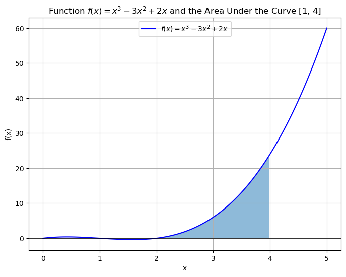
The area under the curve from x=1 to x=4 is 15.75.

---

Problem 2: Partial Derivatives, Chain Rule, and Multiple Integrals

Problem Statement

Let \(z = f(x, y)\) where \(x = u^2 + 3v\) and \(y = uv\).

1. Find the partial derivative of \(z\) with respect to \(u\), denoted as \(\frac{\partial z}{\partial u}\), using the chain rule.

2. Calculate the double integral of \(z(x, y) = x + y\) over the region \(R\), where \(R\) is the square defined by \(0 \leq x \leq 2\) and \(0 \leq y \leq 1\).

Solution:

1. Applying the Chain Rule:

Let \(f(x, y) = x + y\).

To find \(\frac{\partial z}{\partial u}\), use the chain rule:

\[ \frac{\partial z}{\partial u} = \frac{\partial f}{\partial x} \cdot \frac{\partial x}{\partial u} + \frac{\partial f}{\partial y} \cdot \frac{\partial y}{\partial u} \]

For the function \(f(x, y) = x + y\):

\[ \frac{\partial f}{\partial x} = 1, \quad \frac{\partial f}{\partial y} = 1 \]

Next, calculate \(\frac{\partial x}{\partial u}\) and \(\frac{\partial y}{\partial u}\):

Given \(x = u^2 + 3v\) and \(y = uv\):

\[ \frac{\partial x}{\partial u} = 2u, \quad \frac{\partial y}{\partial u} = v \]

Now substitute these into the chain rule equation:

\[ \frac{\partial z}{\partial u} = 1 \cdot 2u + 1 \cdot v = 2u + v \]

Thus, the partial derivative of \(z\) with respect to \(u\) is:

\[ \frac{\partial z}{\partial u} = 2u + v \]

2. Multiple Integrals:

Now, let’s compute the double integral of \(z(x, y) = x + y\) over the region \(R\), defined by \(0 \leq x \leq 2\) and \(0 \leq y \leq 1\).

The integral to solve is:

\[ \int_0^1 \int_0^2 (x + y) \, dx \, dy \]

First, integrate with respect to \(x\):

\[ \int_0^2 (x + y) \, dx = \int_0^2 x \, dx + \int_0^2 y \, dx = \left[ \frac{x^2}{2} \right]_0^2 + \left[ yx \right]_0^2 \]

Evaluating the integrals:

\[ \frac{2^2}{2} - 0 + y(2 - 0) = 2 + 2y \]

Now, integrate with respect to \(y\):

\[ \int_0^1 (2 + 2y) \, dy = \int_0^1 2 \, dy + \int_0^1 2y \, dy = \left[ 2y \right]_0^1 + \left[ y^2 \right]_0^1 \]

Evaluating the integrals:

\[ 2(1 - 0) + (1^2 - 0^2) = 2 + 1 = 3 \]

Thus, the value of the double integral is:

\[ \int_0^1 \int_0^2 (x + y) \, dx \, dy = 3 \]

---

Problem 3: Parametric Equations and Applications

Problem Statement

A particle is moving along a curve defined by the following parametric equations:

\[ x(t) = 3t^2 - 2t \]

\[ y(t) = 2t^3 - t \]

where \(x(t)\) and \(y(t)\) represent the particle’s position at time \(t\).

1. Find the velocity and acceleration vectors of the particle at time \(t\).

2. Determine the time \(t\) when the particle’s velocity is zero.

3. Find the length of the curve traced by the particle between \(t = 0\) and \(t = 2\).

Solution

1. Velocity and Acceleration Vectors

To find the velocity and acceleration, we differentiate the parametric equations with respect to time \(t\).

• Velocity is the derivative of position with respect to time:

  \[ v_x(t) = \frac{dx}{dt} = 6t - 2 \]
  \[ v_y(t) = \frac{dy}{dt} = 6t^2 - 1 \]

  Therefore, the velocity vector at time \(t\) is:

  \[ \mathbf{v}(t) = (6t - 2) \hat{i} + (6t^2 - 1) \hat{j} \]

• Acceleration is the derivative of velocity with respect to time:

  \[ a_x(t) = \frac{d^2x}{dt^2} = 6 \]
  \[ a_y(t) = \frac{d^2y}{dt^2} = 12t \]

  Therefore, the acceleration vector is:

  \[ \mathbf{a}(t) = 6 \hat{i} + 12t \hat{j} \]

2. Time When the Particle’s Velocity is Zero

For the velocity to be zero, both components of the velocity vector must be zero simultaneously:

\[ 6t - 2 = 0 \quad \text{and} \quad 6t^2 - 1 = 0 \]

From \(6t - 2 = 0\), solving for \(t\) gives:

\[ t = \frac{1}{3} \]

Substituting \(t = \frac{1}{3}\) into the second equation:

\[ 6 \left(\frac{1}{3}\right)^2 - 1 = \frac{2}{3} - 1 = -\frac{1}{3} \neq 0 \]

Thus, there is no time \(t\) where the particle’s velocity is exactly zero in both the \(x\) and \(y\) directions.

3. Length of the Curve

The length of the curve traced by the particle from \(t = 0\) to \(t = 2\) is given by the formula:

\[ L = \int_0^2 \sqrt{\left(\frac{dx}{dt}\right)^2 + \left(\frac{dy}{dt}\right)^2} \, dt \]

Substitute the derivatives \(v_x(t) = 6t - 2\) and \(v_y(t) = 6t^2 - 1\):

\[ L = \int_0^2 \sqrt{(6t - 2)^2 + (6t^2 - 1)^2} \, dt \]

This integral can be solved either numerically or using appropriate substitution techniques to find the length of the curve.

Applications

Parametric equations are widely used to describe curves and motions in physics, engineering, and computer graphics. For instance, they are used to model the trajectory of particles, motion along a path, and even design complex curves in computer-aided design (CAD) software.

Python Visualization and Curve Length Calculation:

Here’s the Python code to plot the parametric curve, velocity and acceleration vectors, and calculate the length of the curve numerically:

import numpy as np
import matplotlib.pyplot as plt
from scipy.integrate import quad

# Define the parametric equations for x(t) and y(t)
def x(t):
    return 3 * t**2 - 2 * t

def y(t):
    return 2 * t**3 - t

# Define the velocity components
def v_x(t):
    return 6 * t - 2

def v_y(t):
    return 6 * t**2 - 1

# Define the acceleration components
def a_x(t):
    return 6

def a_y(t):
    return 12 * t

# Define the integrand for the length of the curve
def integrand(t):
    return np.sqrt(v_x(t)**2 + v_y(t)**2)

# Time range for plotting
t_vals = np.linspace(0, 2, 100)
x_vals = x(t_vals)
y_vals = y(t_vals)

# Plot the parametric curve
plt.figure(figsize=(8, 6))
plt.plot(x_vals, y_vals, label='Parametric Curve: Particle Path', color='blue')

# Calculate and plot velocity and acceleration vectors at specific points
t_points = np.array([0, 0.5, 1, 1.5, 2])
v_x_vals = v_x(t_points)
v_y_vals = v_y(t_points)
a_x_vals = np.full_like(t_points, a_x(0))  # a_x is constant, so create an array with the same length
a_y_vals = a_y(t_points)

# Plot velocity vectors
plt.quiver(x(t_points), y(t_points), v_x_vals, v_y_vals, color='green', angles='xy', scale_units='xy', scale=1, label="Velocity Vectors")

# Plot acceleration vectors
plt.quiver(x(t_points), y(t_points), a_x_vals, a_y_vals, color='red', angles='xy', scale_units='xy', scale=1, label="Acceleration Vectors")

# Labels and Title
plt.xlabel('x')
plt.ylabel('y')
plt.title('Particle Motion: Parametric Curve with Velocity and Acceleration Vectors')
plt.grid(True)
plt.legend()
plt.show()

# Calculate the length of the curve numerically using integration
curve_length, _ = quad(integrand, 0, 2)
print(f"The length of the curve traced by the particle between t = 0 and t = 2 is approximately {curve_length:.2f}.")

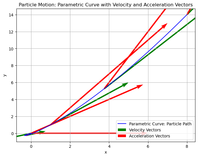
The length of the curve traced by the particle between t = 0 and t = 2 is approximately 17.10.

---

Problem 4: Separable Differential Equation

Solve the following first-order separable ODE:

\[ \frac{dy}{dx} = x^2 + x \]

with the condition \(y(1) = 3\).

Solution:

To solve, integrate both sides with respect to \(x\):

\[ y = \int (x^2 + x) \, dx = \frac{x^3}{3} + \frac{x^2}{2} + C \]

Using the initial condition \(y(1) = 3\), substitute \(x = 1\) and \(y = 3\):

\[ 3 = \frac{1^3}{3} + \frac{1^2}{2} + C \quad \Rightarrow \quad 3 = \frac{1}{3} + \frac{1}{2} + C \]

Solving for \(C\), we get \(C = \frac{13}{6}\), so the solution is:

\[ y(x) = \frac{x^3}{3} + \frac{x^2}{2} + \frac{13}{6} \]

---

Problem 5: Exponential Growth

Solve the differential equation:

\[ \frac{dy}{dx} = e^x + x \]

with the initial condition \(y(0) = 10\).

Solution:

To solve, integrate both sides with respect to \(x\):

\[ y = \int (e^x + x) \, dx = e^x + \frac{x^2}{2} + C \]

Using the initial condition \(y(0) = 10\):

\[ 10 = e^0 + \frac{0^2}{2} + C \quad \Rightarrow \quad 10 = 1 + C \]

Thus, \(C = 9\), and the solution is:

\[ y = e^x + \frac{x^2}{2} + 9 \]

---

Problem 6: Separable Differential Equation

Solve the differential equation

\[ \frac{dy}{dx} = \frac{1}{y}, \qquad y(1) = 2. \]

Solution

Separate variables and integrate:

\[ y \, dy = dx \quad \Longrightarrow \quad \int y \, dy = \int dx \quad \Longrightarrow \quad \frac{y^2}{2} = x + C. \]

Multiply by 2 and absorb constants:

\[ y^2 = 2x + C. \]

Apply the initial condition \(y(1) = 2\):

\[ 4 = 2(1) + C \quad \Longrightarrow \quad C = 2. \]

Hence:

\[ y^2 = 2x + 2. \]

Taking square roots gives \(y = \pm \sqrt{2x+2}\).
Since \(y(1) = 2 > 0\), we select the positive branch:

\[ y(x) = \sqrt{2x+2}, \qquad x > -1. \]

(The negative branch \(y = -\sqrt{2x+2}\) does not satisfy the initial condition.)

---

Problem 7: Linear and Non-Linear Differential Equations

Consider the following two differential equations:

1. Linear Differential Equation:
   Solve the linear first-order differential equation:

   \[ \frac{dy}{dx} + y = e^x \]

2. Non-Linear Differential Equation:
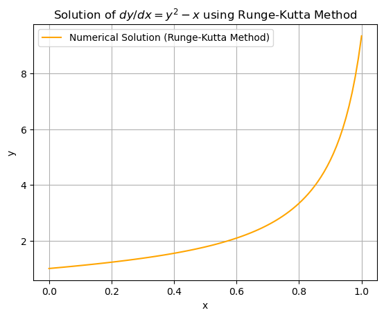
   Solve the non-linear differential equation:

   \[ \frac{dy}{dx} = y^2 - x \]

Solution:

1. Linear Differential Equation

The equation is of the form:

\[ \frac{dy}{dx} + P(x) y = Q(x) \]

where \(P(x) = 1\) and \(Q(x) = e^x\).

Step 1: Find the integrating factor \(\mu(x)\):

\[ \mu(x) = e^{\int P(x) \, dx} = e^{\int 1 \, dx} = e^x \]

Step 2: Multiply both sides of the differential equation by the integrating factor \(\mu(x)\):

\[ e^x \frac{dy}{dx} + e^x y = e^{2x} \]

Step 3: The left-hand side is the derivative of \(e^x y\), so we can rewrite the equation as:

\[ \frac{d}{dx} \left( e^x y \right) = e^{2x} \]

Step 4: Integrate both sides:

\[ e^x y = \int e^{2x} \, dx = \frac{e^{2x}}{2} + C \]

Step 5: Solve for \(y\):

\[ y = \frac{e^x}{2} + Ce^{-x} \]

Thus, the general solution is:

\[ y = \frac{e^x}{2} + Ce^{-x} \]

---

2. Non-Linear Differential Equation

The given equation is:

\[ \frac{dy}{dx} = y^2 - x \]

This is a non-linear differential equation and does not have a straightforward analytical solution. However, it can be solved using numerical methods, such as Euler’s method, or qualitative techniques like direction fields to analyze the behavior of the solutions.

Note

While there is no simple analytic solution to present here, numerical solutions can be computed based on initial conditions.

We use the Runge-Kutta method to solve the differential equation:

\[ \frac{dy}{dx} = y^2 - x \]

Python Code:

import numpy as np
import matplotlib.pyplot as plt

# Function representing the ODE dy/dx = y^2 - x
def dydx(x, y):
    return y**2 - x

# Fourth-order Runge-Kutta method for numerical solution of ODE
def runge_kutta_method(dydx, x0, y0, x_end, h):
    x_values = np.arange(x0, x_end + h, h)
    y_values = np.zeros(len(x_values))
    y_values[0] = y0
    
    for i in range(1, len(x_values)):
        x = x_values[i-1]
        y = y_values[i-1]
        
        k1 = h * dydx(x, y)
        k2 = h * dydx(x + h/2, y + k1/2)
        k3 = h * dydx(x + h/2, y + k2/2)
        k4 = h * dydx(x + h, y + k3)
        
        y_values[i] = y + (k1 + 2*k2 + 2*k3 + k4) / 6
    
    return x_values, y_values

# Adjust the domain to avoid large values causing overflow
x0 = 0  # Initial x
y0 = 1  # Initial y
x_end_new = 1  # Limit the domain to avoid instability
h = 0.01  # Step size

# Solve the ODE using Runge-Kutta method with a smaller domain
x_values_rk_new, y_values_rk_new = runge_kutta_method(dydx, x0, y0, x_end_new, h)

# Plot the solution with the new domain
plt.plot(x_values_rk_new, y_values_rk_new, label="Numerical Solution (Runge-Kutta Method)", color="orange")
plt.xlabel('x')
plt.ylabel('y')
plt.title("Solution of $dy/dx = y^2 - x$ using Runge-Kutta Method")
plt.legend()
plt.grid(True)
plt.show()

---

Problem 8: Boundary Value Problem with Initial Conditions

Solve the following second-order boundary value problem (BVP):

\[ \frac{d^2 y}{dx^2} = -k^2 y \]

with the boundary conditions:

\[ y(0) = 0 \quad \text{and} \quad y(L) = 0 \]

where \(k\) is a constant and \(L\) is the length of the domain.

Solution:

Step 1: General Solution of the ODE

The given equation is a second-order homogeneous linear differential equation with constant coefficients:

\[ \frac{d^2 y}{dx^2} = -k^2 y \]

The characteristic equation for this differential equation is:

\[ r^2 + k^2 = 0 \]

This gives the roots:

\[ r = \pm ik \]

So, the general solution for the differential equation is:

\[ y(x) = C_1 \sin(kx) + C_2 \cos(kx) \]

Step 2: Apply the Boundary Conditions

1. First Boundary Condition: \(y(0) = 0\)

Substitute \(x = 0\) into the general solution:

\[ y(0) = C_1 \sin(0) + C_2 \cos(0) = 0 \quad \Rightarrow \quad C_2 = 0 \]

Thus, the solution simplifies to:

\[ y(x) = C_1 \sin(kx) \]

2. Second Boundary Condition: \(y(L) = 0\)

Now, substitute \(x = L\) into the simplified solution:

\[ y(L) = C_1 \sin(kL) = 0 \]

For non-trivial solutions (i.e., \(C_1 \neq 0\)), we require:

\[ \sin(kL) = 0 \]

This implies:

\[ kL = n\pi \quad \Rightarrow \quad k = \frac{n\pi}{L} \]

where \(n\) is an integer (i.e., \(n = 1, 2, 3, \dots\)).

Step 3: Final Solution

The final solution for the boundary value problem is:

\[ y(x) = C_1 \sin\left( \frac{n\pi}{L} x \right) \]

where \(C_1\) is an arbitrary constant and \(n\) is a positive integer.

---

Problem 9: Vector Field and Gradient

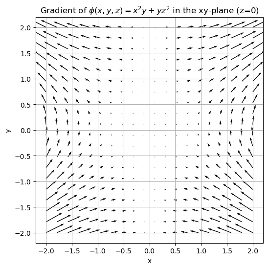
Given the scalar function:

\[ \phi(x, y, z) = x^2 y + yz^2 \]

1. Find the gradient of the scalar field \(\phi(x, y, z)\).

2. Plot the vector field representing the gradient in the \(xy\)-plane for \(z = 0\).

Solution:

1. Gradient of the Scalar Field

The gradient of a scalar field \(\phi(x, y, z)\) is given by:

\[ \nabla \phi = \left( \frac{\partial \phi}{\partial x}, \frac{\partial \phi}{\partial y}, \frac{\partial \phi}{\partial z} \right) \]

For \(\phi(x, y, z) = x^2 y + yz^2\), the partial derivatives are:

\[ \frac{\partial \phi}{\partial x} = 2xy \]

\[ \frac{\partial \phi}{\partial y} = x^2 + z^2 \]

\[ \frac{\partial \phi}{\partial z} = 2yz \]

Thus, the gradient vector field is:

\[ \nabla \phi = (2xy, x^2 + z^2, 2yz) \]

2. Plotting the Gradient Field in the \(xy\)-Plane

Since we’re plotting in the \(xy\)-plane for \(z = 0\), the gradient simplifies to:

\[ \nabla \phi(x, y, 0) = (2xy, x^2, 0) \]

Here is the Python code to plot the vector field in the \(xy\)-plane:

import numpy as np
import matplotlib.pyplot as plt

# Define the scalar field gradient in the xy-plane (z=0)
def grad_phi(x, y):
    grad_x = 2 * x * y
    grad_y = x**2
    return grad_x, grad_y

# Create a grid of points
x_vals = np.linspace(-2, 2, 20)
y_vals = np.linspace(-2, 2, 20)
X, Y = np.meshgrid(x_vals, y_vals)

# Compute the gradient at each point
U, V = grad_phi(X, Y)

# Plot the vector field
plt.figure(figsize=(6, 6))
plt.quiver(X, Y, U, V)
plt.xlabel('x')
plt.ylabel('y')
plt.title('Gradient of $\phi(x, y, z) = x^2 y + yz^2$ in the xy-plane (z=0)')
plt.grid(True)
plt.show()

---

Problem 10: Line, Surface, and Volume Integrals

Problem Statement

1. Line Integral: Given the vector field \(\mathbf{F}(x, y) = (x^2, y^2)\), compute the line integral of \(\mathbf{F} \) along the curve \(C\), where \(C\) is the straight line path from point \((0, 0)\) to point \((1, 1)\).

2. Surface Integral: Compute the surface integral of the vector field \(\mathbf{F}(x, y, z) = (y, z, x)\) over the surface \(S\), where \(S\) is the portion of the plane \(z = 4 - x - y\) in the first octant.

3. Volume Integral: Compute the volume integral of the scalar field \(f(x, y, z) = x + y + z\) over the region \(V\), where \(V\) is the region bounded by the cylinder \(x^2 + y^2 = 1\) and the planes \(z = 0\) and \(z = 3\).

Solution

1. Line Integral

We want to compute the line integral of the vector field \(\mathbf{F}(x, y) = (x^2, y^2)\) along the curve \(C\), a straight line from \((0, 0)\) to \((1, 1)\).

The line integral is given by:

\[ \int_C \mathbf{F} \cdot d\mathbf{r} \]

Parameterizing the line as \(x(t) = t\) and \(y(t) = t\), the differential displacement vector is \(d\mathbf{r} = (1, 1) dt\).

The integral becomes:

\[ \int_0^1 (t^2 + t^2) dt = \int_0^1 2t^2 dt \]

The result can be calculated as:

import numpy as np
from scipy.integrate import quad

# Define the parameterized vector field F along the curve x(t) = t, y(t) = t
def integrand_line(t):
    return 2 * t**2  # (x^2 + y^2) = 2t^2

# Compute the line integral from t = 0 to t = 1
line_integral, _ = quad(integrand_line, 0, 1)
print(f"Line integral: {line_integral:.2f}")

Line integral: 0.67

The line integral of the vector field ( \mathbf{F}(x, y) = (x^2, y^2) ) along the curve is:

\[ \int_C \mathbf{F} \cdot d\mathbf{r} = \frac{2}{3} \]

2. Surface Integral

We are asked to compute the surface integral of the vector field ( \mathbf{F}(x, y, z) = (y, z, x) ) over the surface ( S ), which is the portion of the plane ( z = 4 - x - y ) in the first octant.

We compute \(\displaystyle \iint_S \mathbf F\cdot d\mathbf S\) for \(\mathbf F(x,y,z)=(y,z,x)\) over \(S:\ z=4-x-y\) in the first octant, with upward orientation.

Parameterize by \((x,y)\): $\( \mathbf r(x,y)=(x,\,y,\,4-x-y),\quad \mathbf r_x=(1,0,-1),\ \mathbf r_y=(0,1,-1),\ \mathbf r_x\times\mathbf r_y=(1,1,1). \)$

Then $\( \mathbf F(\mathbf r(x,y))\cdot(\mathbf r_x\times\mathbf r_y) =(y,\,4-x-y,\,x)\cdot(1,1,1) = x+y+(4-x-y)=4. \)$

The projection region is the triangle \(R=\{(x,y):\,0\le x\le 4,\ 0\le y\le 4-x\}\) with area \(\tfrac12\cdot 4\cdot 4=8\). Hence $\( \iint_S \mathbf F\cdot d\mathbf S =\iint_R 4\,dx\,dy =4\cdot 8 =32. \)$

Answer: \(\displaystyle \iint_S \mathbf F\cdot d\mathbf S=32\).

Solve the Surface Integral Numerically

We can use Python to compute the surface integral:

from scipy.integrate import dblquad

# Correct integrand: F(r) · (r_x × r_y) = 4 (constant)
def integrand_surface(y, x):
    return 4.0

# Limits for the triangular region: 0 ≤ x ≤ 4, 0 ≤ y ≤ 4 - x
x_min, x_max = 0, 4
y_min = lambda x: 0
y_max = lambda x: 4 - x

# Compute the surface integral
surface_integral, _ = dblquad(integrand_surface, x_min, x_max, y_min, y_max)
print(f"Surface integral: {surface_integral:.2f}")  

Surface integral: 32.00

3. Volume Integral

We are asked to compute the volume integral of the scalar field \( f(x, y, z) = x + y + z \) over the region \( V \), which is bounded by the cylinder \( x^2 + y^2 = 1 \) and the planes \( z = 0 \) and \( z = 3 \).

Step 1: Volume Integral Formula

The volume integral of a scalar field \( f(x, y, z) \) over a volume \( V \) is given by:

\[ \iiint_V f(x, y, z) \, dV \]

Step 2: Switch to Cylindrical Coordinates

Since the region \( V \) is a cylinder, it’s convenient to switch to cylindrical coordinates:

• \( x = r \cos\theta \)

• \( y = r \sin\theta \)

• \( z = z \)

The volume element in cylindrical coordinates is:

\[ dV = r \, dr \, d\theta \, dz \]

The scalar field \( f(x, y, z) = x + y + z \) becomes:

\[ f(r, \theta, z) = r \cos\theta + r \sin\theta + z \]

Step 3: Set Up the Volume Integral

The region \( V \) is bounded by:

• \( r \in [0, 1] \) (the radius of the cylinder),

• \( \theta \in [0, 2\pi] \) (the full revolution around the cylinder),

• \( z \in [0, 3] \) (the height of the cylinder).

The volume integral in cylindrical coordinates is:

\[ \iiint_V (r \cos\theta + r \sin\theta + z) \, r \, dr \, d\theta \, dz \]

Step 4: Solve the Volume Integral Numerically

We can use Python to compute the volume integral:

from scipy.integrate import tplquad
import numpy as np

# Define the scalar field in cylindrical coordinates f(r, theta, z)
def integrand_volume(z, r, theta):
    return r * (r * np.cos(theta) + r * np.sin(theta) + z)

# Limits for the volume integral
r_min, r_max = 0, 1
theta_min, theta_max = 0, 2 * np.pi
z_min, z_max = 0, 3

# Compute the volume integral
volume_integral, _ = tplquad(integrand_volume, z_min, z_max, r_min, r_max, theta_min, theta_max)
print(f"Volume integral: {volume_integral:.2f}")

Volume integral: 34.07

Step 5: Final Answer

By symmetry, the contributions from \(x\) and \(y\) vanish over the cylinder.
Only the \(z\)-term contributes:

\[ \iiint_V z \, dV = \int_{0}^{2\pi} \int_{0}^{1} \int_{0}^{3} z \, r \, dz \, dr \, d\theta = 2\pi \cdot \left(\tfrac{1}{2}\right) \cdot \left(\tfrac{9}{2}\right) = \tfrac{9\pi}{2}. \]

Thus, the correct result of the volume integral is:

\[ \iiint_V (x + y + z) \, dV = \tfrac{9\pi}{2}. \]

---

Problem 11: Application of the Divergence Theorem and Stokes’ Theorem in Fluid Flow

Problem Statement:

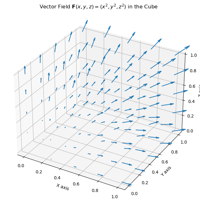
1. Divergence Theorem: Given the vector field \( \mathbf{F}(x, y, z) = (x^2, y^2, z^2) \), use the Divergence Theorem to compute the flux of \( \mathbf{F} \) through the surface of the cube bounded by the planes \( x = 0 \), \( x = 1 \), \( y = 0 \), \( y = 1 \), \( z = 0 \), and \( z = 1 \).

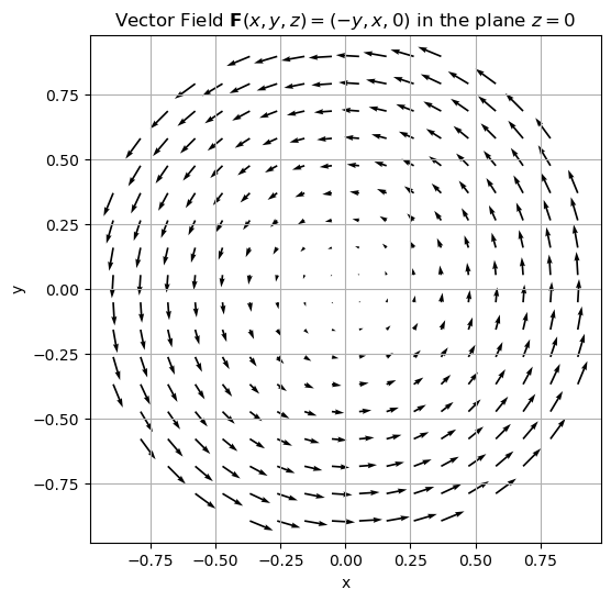
2. Stokes’ Theorem: Given the vector field \( \mathbf{F}(x, y, z) = (-y, x, 0) \), use Stokes’ Theorem to compute the circulation of \( \mathbf{F} \) around the boundary of the surface defined by the disk \( x^2 + y^2 \leq 1 \) in the plane \( z = 0 \).

Solution

1. Divergence Theorem:

The Divergence Theorem relates the flux of a vector field through a closed surface to the volume integral of the divergence of the vector field over the region enclosed by the surface. Mathematically, it states:

\[ \iint_S \mathbf{F} \cdot d\mathbf{A} = \iiint_V (\nabla \cdot \mathbf{F}) \, dV \]

where \( \mathbf{F} \) is the vector field, \( d\mathbf{A} \) is the surface area element, and \( \nabla \cdot \mathbf{F} \) is the divergence of \( \mathbf{F} \).

Step 1: Compute the divergence of the vector field \( \mathbf{F}(x, y, z) = (x^2, y^2, z^2) \):

\[ \nabla \cdot \mathbf{F} = \frac{\partial}{\partial x}(x^2) + \frac{\partial}{\partial y}(y^2) + \frac{\partial}{\partial z}(z^2) = 2x + 2y + 2z \]

Step 2: Set up the volume integral over the cube \( 0 \leq x \leq 1 \), \( 0 \leq y \leq 1 \), and \( 0 \leq z \leq 1 \):

\[ \iiint_V (2x + 2y + 2z) \, dV = \int_0^1 \int_0^1 \int_0^1 (2x + 2y + 2z) \, dx \, dy \, dz \]

Step 3: Compute the integral:

1. Integrating with respect to \( x \):

\[ \int_0^1 (2x + 2y + 2z) \, dx = \left[ x^2 + 2yx + 2zx \right]_0^1 = 1 + 2y + 2z \]

2. Integrating with respect to \( y \):

\[ \int_0^1 (1 + 2y + 2z) \, dy = \left[ y + y^2 + 2zy \right]_0^1 = 1 + 1 + 2z = 2 + 2z \]

3. Finally, integrate with respect to \( z \):

\[ \int_0^1 (2 + 2z) \, dz = \left[ 2z + z^2 \right]_0^1 = 2 + 1 = 3 \]

Thus, the flux of \( \mathbf{F} \) through the surface of the cube is:

\[ \iint_S \mathbf{F} \cdot d\mathbf{A} = 3 \]

Python

We will create a grid of points in the cube and define the vector field \( \mathbf{F}(x, y, z) = (x^2, y^2, z^2) \) on this grid.

import numpy as np
import matplotlib.pyplot as plt

# Create a grid of points in the cube
x_vals, y_vals, z_vals = np.linspace(0, 1, 5), np.linspace(0, 1, 5), np.linspace(0, 1, 5)
X, Y, Z = np.meshgrid(x_vals, y_vals, z_vals)


# Define the vector field F(x, y, z) = (x^2, y^2, z^2)
# Vector field components
F_x = X**2  # x component of the vector field
F_y = Y**2  # y component of the vector field
F_z = Z**2  # z component of the vector field

# Plot the vector field using quiver
fig = plt.figure(figsize=(8, 8))
ax = fig.add_subplot(111, projection='3d')
ax.quiver(X, Y, Z, F_x, F_y, F_z, length=0.1)

# Set labels
ax.set_xlabel('X axis')
ax.set_ylabel('Y axis')
ax.set_zlabel('Z axis')
ax.set_title('Vector Field $\\mathbf{F}(x, y, z) = (x^2, y^2, z^2)$ in the Cube')

plt.show()

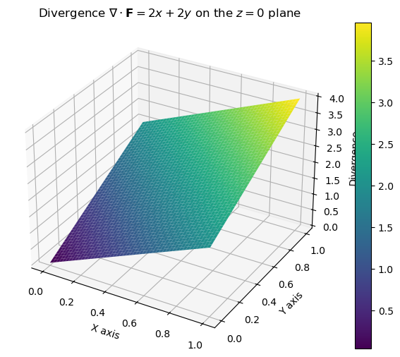
Plot of the divergence field at \(Z=0\)

import numpy as np
import matplotlib.pyplot as plt
from mpl_toolkits.mplot3d import Axes3D

# Create a grid of points in the cube
n = 50  # Increase the grid density for a smoother surface plot
x_vals, y_vals = np.linspace(0, 1, n), np.linspace(0, 1, n)
X, Y = np.meshgrid(x_vals, y_vals)

# Calculate the divergence at z = 0 plane
Divergence_z0 = 2 * X + 2 * Y  # Since z = 0, the divergence simplifies to 2x + 2y

# Create a 3D surface plot for the divergence on z = 0 plane
fig = plt.figure(figsize=(8, 6))
ax = fig.add_subplot(111, projection='3d')

# Plot the surface
surface_plot = ax.plot_surface(X, Y, Divergence_z0, cmap='viridis', edgecolor='none')

# Add a color bar
fig.colorbar(surface_plot, ax=ax)

# Set labels
ax.set_xlabel('X axis')
ax.set_ylabel('Y axis')
ax.set_zlabel('Divergence')
ax.set_title('Divergence $\\nabla \\cdot \\mathbf{F} = 2x + 2y$ on the $z = 0$ plane')

plt.show()

Volume integral for computing the divergence

from scipy.integrate import tplquad

# Define the divergence of the vector field
def divergence(x, y, z):
    return 2 * x + 2 * y + 2 * z

# Limits of the cube: x, y, z in [0, 1]
volume_integral, _ = tplquad(divergence, 0, 1, lambda x: 0, lambda x: 1, lambda x, y: 0, lambda x, y: 1)
print(f"Volume integral of the divergence: {volume_integral:.2f}")

Volume integral of the divergence: 3.00

2. Stokes’ Theorem

Stokes’ Theorem relates the circulation of a vector field around a closed curve to the surface integral of the curl of the vector field over the surface bounded by the curve. Mathematically, it states:

\[ \oint_C \mathbf{F} \cdot d\mathbf{r} = \iint_S (\nabla \times \mathbf{F}) \cdot d\mathbf{A} \]

where \( C \) is the boundary curve, and \( S \) is the surface bounded by \( C \).

Step 1: Compute the curl of the vector field \( \mathbf{F}(x, y, z) = (-y, x, 0) \):

\[ \nabla \times \mathbf{F} = \left( \frac{\partial}{\partial y}(0) - \frac{\partial}{\partial z}(x), \frac{\partial}{\partial z}(-y) - \frac{\partial}{\partial x}(0), \frac{\partial}{\partial x}(x) - \frac{\partial}{\partial y}(-y) \right) = (0, 0, 2) \]

The curl of \( \mathbf{F} \) is \( (0, 0, 2) \).

Step 2: The surface is the disk \( x^2 + y^2 \leq 1 \) in the plane \( z = 0 \). The area element for a flat disk is \( dA = dx \, dy \).

Thus, the surface integral becomes:

\[ \iint_S (0, 0, 2) \cdot (0, 0, 1) \, dA = 2 \iint_S dA \]

Step 3: The area of the disk is:

\[ \iint_S dA = \pi (1^2) = \pi \]

Therefore, the circulation of \( \mathbf{F} \) around the boundary of the disk is:

\[ \oint_C \mathbf{F} \cdot d\mathbf{r} = 2\pi \]

Python

Visualize the vector field

import numpy as np
import matplotlib.pyplot as plt

# Define the grid for the disk x^2 + y^2 <= 1
x_vals = np.linspace(-1, 1, 20)
y_vals = np.linspace(-1, 1, 20)
X, Y = np.meshgrid(x_vals, y_vals)

# Mask the points that lie outside the disk (x^2 + y^2 > 1)
mask = X**2 + Y**2 <= 1
X = X[mask]
Y = Y[mask]

# Define the vector field F(x, y, z) = (-y, x, 0) at z = 0
U = -Y  # x-component of the vector field
V = X   # y-component of the vector field

# Plot the vector field
plt.figure(figsize=(6,6))
plt.quiver(X, Y, U, V)
plt.title("Vector Field $\\mathbf{F}(x, y, z) = (-y, x, 0)$ in the plane $z = 0$")
plt.xlabel('x')
plt.ylabel('y')
plt.grid(True)
plt.axis('equal')
plt.show()

Plot the Boundary Curve: The boundary curve of the disk is the unit circle

import matplotlib.pyplot as plt

# Define the boundary curve (circle) x^2 + y^2 = 1
theta = np.linspace(0, 2*np.pi, 100)
x_circle = np.cos(theta)
y_circle = np.sin(theta)

# Plot the vector field and the boundary curve
plt.figure(figsize=(6,6))
plt.quiver(X, Y, U, V, color='blue', alpha=0.6)
plt.plot(x_circle, y_circle, color='red', linewidth=2, label='Boundary Curve')
plt.title("Vector Field and Boundary Curve $x^2 + y^2 = 1$")
plt.xlabel('x')
plt.ylabel('y')
plt.legend()
plt.grid(True)
plt.axis('equal')
plt.show()

Calculate the Curl

# Area of the disk
area_of_disk = np.pi * 1**2  # radius = 1
curl_z = 2  # curl in the z direction

# Surface integral of the curl
surface_integral = curl_z * area_of_disk
print(f"Surface integral of the curl: {surface_integral:.2f}")

Surface integral of the curl: 6.28

Problem 12: Motion on an Inclined Plane

A block of mass \( m = 5 \, \text{kg} \) is placed on a frictionless inclined plane, which makes an angle of \( \theta = 30^\circ \) with the horizontal. The block is released from rest at the top of the incline.

1. What is the acceleration of the block along the incline?

2. How fast is the block moving after 2 seconds?

3. How far down the incline has the block moved after 2 seconds?

Solution

1. Acceleration Along the Incline

Using Newton’s second law of motion, the net force acting on the block along the incline is the component of the gravitational force that acts parallel to the incline. Since the plane is frictionless, the only force along the incline is due to gravity:

\[ F_{\parallel} = mg \sin \theta \]

According to Newton’s second law, \( F = ma \), so the acceleration along the incline is:

\[ a = \frac{F_{\parallel}}{m} = \frac{mg \sin \theta}{m} = g \sin \theta \]

Substituting the values:

\[ a = (9.8 \, \text{m/s}^2) \sin 30^\circ = (9.8 \, \text{m/s}^2) \times 0.5 = 4.9 \, \text{m/s}^2 \]

Thus, the acceleration of the block along the incline is:

\[ a = 4.9 \, \text{m/s}^2 \]

2. Speed After 2 Seconds

The block is released from rest, so its initial velocity is \( v_0 = 0 \, \text{m/s} \). Using the equation of motion:

\[ v = v_0 + at \]

Substitute the known values:

\[ v = 0 + (4.9 \, \text{m/s}^2) \times 2 \, \text{s} = 9.8 \, \text{m/s} \]

Thus, after 2 seconds, the speed of the block is:

\[ v = 9.8 \, \text{m/s} \]

3. Distance Traveled After 2 Seconds

We can use the equation of motion:

\[ s = v_0 t + \frac{1}{2} a t^2 \]

Substitute the known values:

\[ s = 0 \times 2 + \frac{1}{2} (4.9 \, \text{m/s}^2) (2 \, \text{s})^2 = \frac{1}{2} (4.9 \, \text{m/s}^2) \times 4 = 9.8 \, \text{m} \]

Thus, the block travels a distance of:

\[ s = 9.8 \, \text{m} \]

Summary

1. The acceleration along the incline is \( 4.9 \, \text{m/s}^2 \).

2. The speed after 2 seconds is \( 9.8 \, \text{m/s} \).

3. The distance traveled after 2 seconds is \( 9.8 \, \text{m} \).

---

Problem 13: Object in Uniform Circular Motion with Angular Velocity

A car of mass \(m = 1000 \, \text{kg}\) is moving in a circular track of radius \(r = 50 \, \text{m}\) with a constant speed of \(v = 20 \, \text{m/s}\).

1. What is the magnitude of the centripetal force acting on the car?

2. What is the angular velocity of the car?

3. If the coefficient of static friction between the tires and the track is \(\mu_s = 0.6\), what is the maximum speed the car can have before it starts to skid?

Solution

1. Magnitude of the Centripetal Force

In uniform circular motion, the centripetal force is the force that keeps an object moving in a circular path and is directed towards the center of the circle. The formula for centripetal force is:

\[ F_c = \frac{mv^2}{r} \]

where:

• \(m = 1000 \, \text{kg}\) is the mass of the car,

• \(v = 20 \, \text{m/s}\) is the speed of the car,

• \(r = 50 \, \text{m}\) is the radius of the circular path.

Substituting the known values:

\[ F_c = \frac{(1000 \, \text{kg}) \times (20 \, \text{m/s})^2}{50 \, \text{m}} = \frac{1000 \times 400}{50} = 8000 \, \text{N} \]

Thus, the magnitude of the centripetal force is:

\[ F_c = 8000 \, \text{N} \]

2. Angular Velocity of the Car

The angular velocity \( \omega \) of an object in circular motion is related to its linear velocity \(v\) by the following relationship:

\[ \omega = \frac{v}{r} \]

where:

• \(v = 20 \, \text{m/s}\) is the linear velocity of the car,

• \(r = 50 \, \text{m}\) is the radius of the circular path.

Substituting the known values:

\[ \omega = \frac{20 \, \text{m/s}}{50 \, \text{m}} = 0.4 \, \text{rad/s} \]

Thus, the angular velocity of the car is:

\[ \omega = 0.4 \, \text{rad/s} \]

3. Maximum Speed Before Skidding

The car will start to skid when the frictional force between the tires and the track is no longer sufficient to provide the necessary centripetal force. The maximum frictional force (which acts as the centripetal force) is given by:

\[ F_f = \mu_s F_n \]

where:

• \(\mu_s = 0.6\) is the coefficient of static friction,

• \(F_n = mg\) is the normal force, where \(g = 9.8 \, \text{m/s}^2\) is the acceleration due to gravity.

Substituting the known values:

\[ F_f = \mu_s mg = 0.6 \times 1000 \, \text{kg} \times 9.8 \, \text{m/s}^2 = 5880 \, \text{N} \]

The maximum centripetal force that friction can provide is \(F_f = 5880 \, \text{N}\). This force is also equal to the centripetal force required for circular motion, so we can set it equal to the formula for centripetal force and solve for the maximum speed \(v_\text{max}\):

\[ F_f = \frac{m v_\text{max}^2}{r} \]

Substitute the values for \(F_f\), \(m\), and \(r\):

\[ 5880 \, \text{N} = \frac{1000 \, \text{kg} \times v_\text{max}^2}{50 \, \text{m}} \]

Solving for \(v_\text{max}\):

\[ v_\text{max}^2 = \frac{5880 \times 50}{1000} = 294 \]

\[ v_\text{max} = \sqrt{294} \approx 17.15 \, \text{m/s} \]

Thus, the maximum speed the car can have before skidding is:

\[ v_\text{max} \approx 17.15 \, \text{m/s} \]

Summary of Results

1. The magnitude of the centripetal force acting on the car is \(8000 \, \text{N}\).

2. The angular velocity of the car is \(0.4 \, \text{rad/s}\).

3. The maximum speed the car can have before it starts to skid is approximately \(17.15 \, \text{m/s}\).

---

Problem 14: Elastic Collision and Energy Conservation

A ball of mass \(m_1 = 2 \, \text{kg}\) is moving with a velocity of \(v_1 = 5 \, \text{m/s}\) towards another stationary ball of mass \(m_2 = 3 \, \text{kg}\). The collision between the two balls is perfectly elastic.

1. What are the velocities of the two balls after the collision?

2. Verify that both momentum and kinetic energy are conserved in the system.

Solution

1. Final Velocities of the Balls After the Collision

In a perfectly elastic collision, both momentum and kinetic energy are conserved.

Conservation of Momentum

The total momentum before the collision must equal the total momentum after the collision. The equation for conservation of momentum is:

\[ m_1 v_1 + m_2 v_2 = m_1 v_1' + m_2 v_2' \]

Where:

• \(v_1' \) is the velocity of ball 1 after the collision,

• \(v_2' \) is the velocity of ball 2 after the collision,

• \(v_2 = 0\) since ball 2 is initially at rest.

Thus, the momentum conservation equation simplifies to:

\[ m_1 v_1 = m_1 v_1' + m_2 v_2' \]

Substitute the known values for \(m_1\), \(v_1\), and \(m_2\):

\[ 2 \, \text{kg} \times 5 \, \text{m/s} = 2 \, \text{kg} \times v_1' + 3 \, \text{kg} \times v_2' \]

\[ 10 \, \text{kg} \cdot \text{m/s} = 2 v_1' + 3 v_2' \]

Conservation of Kinetic Energy

The total kinetic energy before the collision must equal the total kinetic energy after the collision. The equation for conservation of kinetic energy is:

\[ \frac{1}{2} m_1 v_1^2 + \frac{1}{2} m_2 v_2^2 = \frac{1}{2} m_1 v_1'^2 + \frac{1}{2} m_2 v_2'^2 \]

Since \(v_2 = 0\), this simplifies to:

\[ \frac{1}{2} m_1 v_1^2 = \frac{1}{2} m_1 v_1'^2 + \frac{1}{2} m_2 v_2'^2 \]

Substitute the known values:

\[ \frac{1}{2} \times 2 \, \text{kg} \times (5 \, \text{m/s})^2 = \frac{1}{2} \times 2 \, \text{kg} \times v_1'^2 + \frac{1}{2} \times 3 \, \text{kg} \times v_2'^2 \]

\[ 25 \, \text{J} = v_1'^2 + 1.5 v_2'^2 \]

Now, we have two equations:

1. \( 10 = 2 v_1' + 3 v_2' \)

2. \( 25 = v_1'^2 + 1.5 v_2'^2 \)

We can solve this system of equations to find \(v_1'\) and \(v_2'\).

Solving the System of Equations

From the momentum equation:

\[ v_1' = 5 - 1.5 v_2' \]

Substitute this into the energy equation:

\[ 25 = (5 - 1.5 v_2')^2 + 1.5 v_2'^2 \]

Expand and simplify:

\[ 25 = (25 - 15 v_2' + 2.25 v_2'^2) + 1.5 v_2'^2 \]

\[ 25 = 25 - 15 v_2' + 3.75 v_2'^2 \]

Simplifying further:

\[ 0 = -15 v_2' + 3.75 v_2'^2 \]

Factor out \(v_2'\):

\[ v_2' (3.75 v_2' - 15) = 0 \]

Thus, \(v_2' = 0\) or \(v_2' = 4 \, \text{m/s}\).

If \(v_2' = 0\), the collision would not have been elastic, so \(v_2' = 4 \, \text{m/s}\).

Now, substitute \(v_2' = 4 \, \text{m/s}\) into the momentum equation:

\[ v_1' = 5 - 1.5 \times 4 = 5 - 6 = -1 \, \text{m/s} \]

Thus, the velocities after the collision are:

• \(v_1' = -1 \, \text{m/s}\) (ball 1 reverses direction),

• \(v_2' = 4 \, \text{m/s}\) (ball 2 moves forward).

2. Verifying Conservation of Momentum and Energy

Momentum Conservation

Before the collision:

\[ p_\text{initial} = m_1 v_1 + m_2 v_2 = 2 \times 5 + 3 \times 0 = 10 \, \text{kg} \cdot \text{m/s} \]

After the collision:

\[ p_\text{final} = m_1 v_1' + m_2 v_2' = 2 \times (-1) + 3 \times 4 = -2 + 12 = 10 \, \text{kg} \cdot \text{m/s} \]

Momentum is conserved, as \(p_\text{initial} = p_\text{final}\).

Energy Conservation

Before the collision:

\[ KE_\text{initial} = \frac{1}{2} m_1 v_1^2 = \frac{1}{2} \times 2 \times (5)^2 = 25 \, \text{J} \]

After the collision:

\[ KE_\text{final} = \frac{1}{2} m_1 v_1'^2 + \frac{1}{2} m_2 v_2'^2 = \frac{1}{2} \times 2 \times (-1)^2 + \frac{1}{2} \times 3 \times (4)^2 \]

\[ KE_\text{final} = 1 + 24 = 25 \, \text{J} \]

Energy is conserved, as \(KE_\text{initial} = KE_\text{final}\).

Summary of Results

1. After the collision, ball 1 has a velocity of \(v_1' = -1 \, \text{m/s}\) and ball 2 has a velocity of \(v_2' = 4 \, \text{m/s}\).

2. Both momentum and kinetic energy are conserved in this elastic collision.

---

Problem 15: Object Falling from a Height (Energy Conservation)

A rock of mass \(m = 2 \, \text{kg}\) is dropped from a height of \(h = 10 \, \text{m}\) above the ground. Assume no air resistance.

1. What is the speed of the rock just before it hits the ground?

2. Verify that the potential energy at the start equals the kinetic energy just before impact.

3. How long does it take for the rock to hit the ground?

Solution

This problem involves the conversion of gravitational potential energy into kinetic energy as the rock falls. We will also verify that energy is conserved in the system.

1. Speed of the Rock Just Before Impact

To find the speed of the rock just before it hits the ground, we use the conservation of mechanical energy. Initially, the rock has gravitational potential energy, and as it falls, this energy is converted into kinetic energy.

The total mechanical energy of the rock at the top (just before it is dropped) is:

\[ E_\text{total} = PE_\text{initial} = mgh \]

Where:

• \(m = 2 \, \text{kg}\) is the mass of the rock,

• \(g = 9.8 \, \text{m/s}^2\) is the acceleration due to gravity,

• \(h = 10 \, \text{m}\) is the height from which the rock is dropped.

Substituting the known values:

\[ PE_\text{initial} = 2 \, \text{kg} \times 9.8 \, \text{m/s}^2 \times 10 \, \text{m} = 196 \, \text{J} \]

At the moment just before the rock hits the ground, all the potential energy has been converted into kinetic energy. The total mechanical energy of the rock just before impact is:

\[ E_\text{total} = KE_\text{final} = \frac{1}{2} m v^2 \]

Since energy is conserved, \(PE_\text{initial} = KE_\text{final}\). So:

\[ mgh = \frac{1}{2} m v^2 \]

Cancel the mass \(m\) on both sides of the equation:

\[ gh = \frac{1}{2} v^2 \]

Solving for \(v\):

\[ v^2 = 2gh \]

Substitute the values of \(g\) and \(h\):

\[ v^2 = 2 \times 9.8 \, \text{m/s}^2 \times 10 \, \text{m} = 196 \, \text{m}^2/\text{s}^2 \]

Taking the square root:

\[ v = \sqrt{196} = 14 \, \text{m/s} \]

Thus, the speed of the rock just before it hits the ground is:

\[ v = 14 \, \text{m/s} \]

2. Verify Energy Conservation

Initially, the rock has only potential energy:

\[ PE_\text{initial} = mgh = 196 \, \text{J} \]

Just before the rock hits the ground, all this potential energy is converted into kinetic energy. The final kinetic energy is:

\[ KE_\text{final} = \frac{1}{2} m v^2 = \frac{1}{2} \times 2 \, \text{kg} \times (14 \, \text{m/s})^2 = \frac{1}{2} \times 2 \times 196 = 196 \, \text{J} \]

Since \(PE_\text{initial} = KE_\text{final}\), energy is conserved in the system.

3. Time to Hit the Ground

To find how long it takes for the rock to hit the ground, we use the equation for vertical motion under constant acceleration:

\[ h = \frac{1}{2} g t^2 \]

Solving for \(t\):

\[ t^2 = \frac{2h}{g} \]

Substitute the values for \(h\) and \(g\):

\[ t^2 = \frac{2 \times 10 \, \text{m}}{9.8 \, \text{m/s}^2} \approx 2.04 \, \text{s}^2 \]

Taking the square root:

\[ t = \sqrt{2.04} \approx 1.43 \, \text{s} \]

Thus, it takes approximately:

\[ t \approx 1.43 \, \text{s} \]

for the rock to hit the ground.

Summary of Results

1. The speed of the rock just before it hits the ground is \(14 \, \text{m/s}\).

2. The potential energy at the start equals the kinetic energy just before impact, confirming that energy is conserved.

3. It takes approximately \(1.43 \, \text{seconds}\) for the rock to hit the ground.