Components of the Climate System#
The climate system is a complex, interconnected web of five main components: the atmosphere, hydrosphere, cryosphere, lithosphere, and biosphere. Each plays a unique role in maintaining Earth’s climate, but they’re all constantly interacting and influencing one another. Let’s break down these components, along with some of the challenges in monitoring them.
1. Atmosphere#

The atmosphere is the layer of gases surrounding Earth, where weather happens and where greenhouse gases trap heat, keeping the planet warm enough for life. It’s crucial for distributing heat through winds and weather patterns, which helps balance temperatures globally.
Monitoring Challenges:
Tracking changes in the atmosphere is tough due to its dynamic nature. While satellites provide global coverage, they can’t measure every detail. Ground stations, balloons, and planes provide more localized data, but this data can be patchy. Moreover, measuring trace gases like CO₂ and methane precisely over time and space is challenging. Atmospheric monitoring also requires constant updates due to rapid changes, especially with pollutants and short-lived greenhouse gases.
2. Hydrosphere#

The hydrosphere includes all water on Earth, like oceans, rivers, and lakes. Oceans, in particular, play a huge role by absorbing heat from the sun and distributing it globally through currents. They also store and release gases like CO₂, influencing atmospheric composition and temperature.
Monitoring Challenges:
Oceans are vast, and monitoring them accurately requires both surface and deep-water data. Satellites can measure surface temperatures and wave heights but can’t see below the surface. Buoys, ships, and underwater sensors provide deeper insights, yet they only cover specific areas, leaving gaps in data. Additionally, the sheer scale and remote locations of many water bodies make it costly and logistically challenging to monitor continuously.
3. Cryosphere#
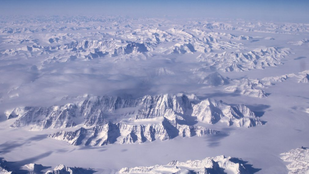
The cryosphere is made up of all frozen water on Earth, including glaciers, ice caps, and snow cover. It plays a crucial role in reflecting sunlight back into space (albedo effect), which helps regulate global temperatures. As temperatures rise, melting ice reduces this reflective cover, leading to more warming—a feedback loop.
Monitoring Challenges:
Observing the cryosphere is difficult because much of it is located in remote or harsh environments, like the Arctic and Antarctic. While satellites can monitor ice cover and movement, they can struggle with accuracy in cloudy conditions or in measuring ice thickness. Field research is challenging and dangerous due to extreme weather and limited accessibility. Climate change has made cryosphere monitoring even more critical, yet logistics and funding limit detailed observations.
4. Lithosphere#
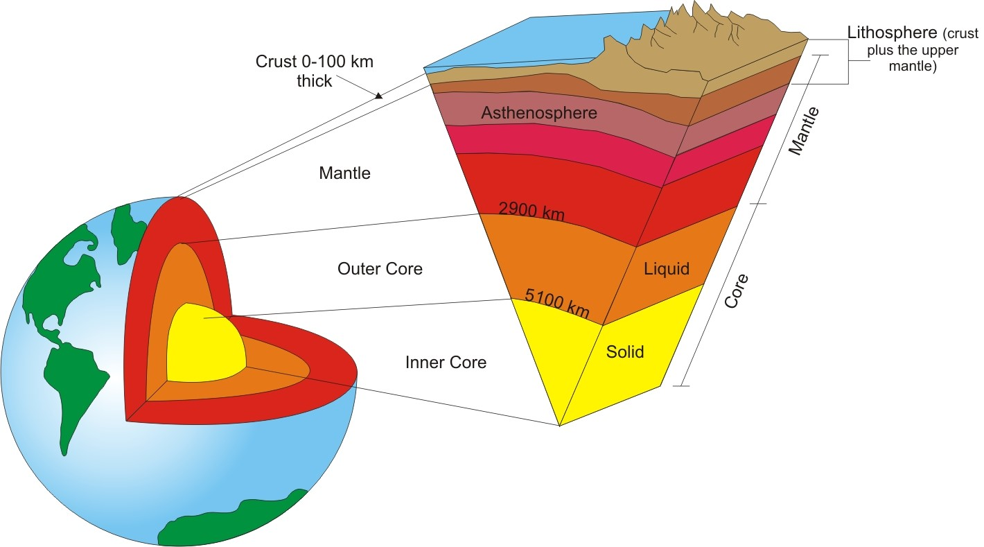
The lithosphere includes Earth’s crust and upper mantle. While it might not seem as active in climate processes, it plays a role by storing carbon in rocks and soils, and its physical characteristics influence local climate (e.g., deserts, mountains).
Monitoring Challenges:
Studying the lithosphere’s impact on climate often involves long-term geological studies, which can be slow and expensive. Carbon fluxes from soils and the weathering of rocks happen over extended periods, making it hard to capture immediate data. Additionally, human land use—like deforestation and urbanization—changes the lithosphere and affects local and global climate, making consistent monitoring even more complicated.
5. Biosphere#
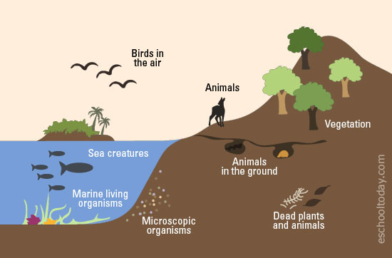
The biosphere encompasses all living organisms. Plants, for example, absorb CO₂ during photosynthesis, which helps regulate greenhouse gas levels. Forests, soils, and oceans serve as carbon sinks, capturing and storing carbon to balance atmospheric levels.
Monitoring Challenges:
The biosphere is incredibly diverse, and monitoring its role in the climate system is complex. Tracking carbon fluxes in forests, soils, and oceans requires vast amounts of data. Deforestation, agriculture, and urbanization add to the challenge, as they alter natural carbon cycles. Remote sensing helps, but it can only measure vegetation cover and health to a limited extent. Understanding detailed biosphere-climate interactions, especially with smaller or underground organisms, remains a challenging area of climate science.
Putting it All Together#
Each component of the climate system presents unique monitoring challenges due to scale, accessibility, and the dynamic nature of these processes. Combining data from satellites, ground stations, buoys, and fieldwork helps create a more complete picture, but gaps and limitations still exist. The rapid pace of climate change makes monitoring these components critical, yet the technological, logistical, and financial challenges are ongoing hurdles for climate scientists worldwide.
Understanding and tracking these components together is crucial for accurate climate models and predictions. The more we learn about how each part functions and interacts, the better we can predict future climate changes and devise strategies to mitigate and adapt to these changes.
Python#
One could use Python in various ways to explore and analyze the concepts in this chapter on climate system components. Using Python to interact with real-world datasets lets you explore each climate system component in depth. Libraries like xarray, matplotlib, and numpy are powerful tools to analyze, visualize, and better understand climate data, bridging the theoretical concepts in the textbook with actual data and observable trends.
Here are some potential examples that tie into each component of the climate system:
1. Atmosphere: Visualizing and Analyzing Atmospheric Data#
Example 1: Load and plot global temperature and pressure data from reanalysis datasets like NCEP/NCAR or ERA5 using
xarrayandmatplotlib. You could plot temperature profiles by latitude or create a time series of atmospheric CO₂ concentrations to see seasonal trends.Example 2: Calculate annual mean temperatures or anomalies to observe trends. For instance, plot temperature changes over time to analyze warming trends across different latitudes.
Example 3: Use
scipyandnumpyto calculate basic atmospheric properties, such as lapse rate or pressure at various altitudes based on the standard atmosphere equations.
2. Hydrosphere: Working with Ocean Data#
Example 1: Use
xarrayandnetCDF4to access sea surface temperature (SST) data from sources like NOAA or NASA. You could visualize SST changes over time, focusing on specific regions, or track seasonal SST patterns.Example 2: Calculate global ocean heat content by integrating ocean temperature across depths. This can provide insights into ocean warming over time and by depth.
Example 3: Plot ocean currents using vector fields. Many reanalysis datasets include u (east-west) and v (north-south) components of current data, allowing you to create vector maps showing the direction and strength of ocean currents.
3. Cryosphere: Analyzing Ice and Snow Data#
Example 1: Load sea ice extent data from sources like NSIDC (National Snow and Ice Data Center) and plot monthly or yearly sea ice extent in the Arctic or Antarctic to observe seasonal cycles and long-term trends.
Example 2: Use snow cover data to visualize snow accumulation and melting patterns throughout the year. For example, plot the extent of snow cover by month to see how it changes with the seasons.
Example 3: Calculate the albedo effect of ice-covered versus ice-free areas by combining albedo data with sea ice cover. This can help visualize how the loss of ice impacts Earth’s energy balance.
4. Lithosphere: Examining Land and Soil Characteristics#
Example 1: Use global or regional datasets to visualize land surface temperature (LST) and understand how it differs from air temperature. For instance, plot LST for various land types (forests, deserts, cities) to see how they absorb and release heat.
Example 2: Analyze soil moisture data from satellite sources, such as SMAP (Soil Moisture Active Passive) to understand the impact of soil moisture on local climates. You could also calculate changes in soil moisture over time to see how droughts or rainfall patterns shift.
Example 3: Explore carbon storage in soils and vegetation by analyzing carbon flux data. For example, use datasets on soil carbon to plot carbon storage across different land types or latitudes.
5. Biosphere: Investigating Vegetation and Carbon Fluxes#
Example 1: Use
xarrayto visualize vegetation indices like NDVI (Normalized Difference Vegetation Index) or EVI (Enhanced Vegetation Index) to monitor plant health and growth. These indices can help track seasonal changes in vegetation and assess the impact of droughts or land use changes.Example 2: Plot carbon fluxes between the biosphere and atmosphere using datasets like FLUXNET, which provides data from flux towers measuring CO₂, water vapor, and energy fluxes in ecosystems. This data can help you visualize how forests, wetlands, or grasslands act as carbon sinks.
Example 3: Analyze seasonal photosynthesis patterns by examining CO₂ uptake and release in different regions. You could plot CO₂ levels in relation to photosynthesis to show the biosphere’s role in regulating atmospheric CO₂.
Putting It All Together: Climate System Analysis#
Example 1: Create a multi-panel plot to show trends in key climate indicators from each component, such as atmospheric CO₂, SST, sea ice extent, land surface temperature, and NDVI. This kind of visualization helps connect the components visually.
Example 2: Perform a correlation analysis between different components. For example, you could analyze the relationship between SST anomalies and atmospheric temperatures or the correlation between sea ice extent and albedo.
Example 3: Build a simple energy balance model in Python. This could involve calculating incoming and outgoing radiation, incorporating albedo from the cryosphere, and visualizing how different components contribute to Earth’s energy balance.