Tropical Thermodynamics & Static Stability#
Lecture 0: Introduction#
At its core, climate emerges from the interplay between water in all its phases and external energy supplied primarily by the Sun.
Our goal is to study the behaviour of the Earth’s climate system on timescales longer than individual weather events.
A fundamental question is: what do we call “climate” and what questions are we trying to answer? Unlike weather, which fluctuates over hours or days, climate refers to long‑term statistics (means, extremes and patterns) of the atmosphere–ocean system.
Climatology is inherently multidisciplinary. It draws on thermodynamics and fluid dynamics to describe the atmosphere and ocean, energy‑balance principles to track radiation and heat, microphysics of clouds and aerosols, and turbulence and chaos theory to understand variability and predictability. Because the climate system comprises interacting subsystems — the continents, oceans, atmosphere, cryosphere, biosphere, lithosphere, and increasingly, human activities — it behaves as a complex set of fluids subject to both oscillations (internal variability) and forcings (natural and anthropogenic). As examples, climate depends on:
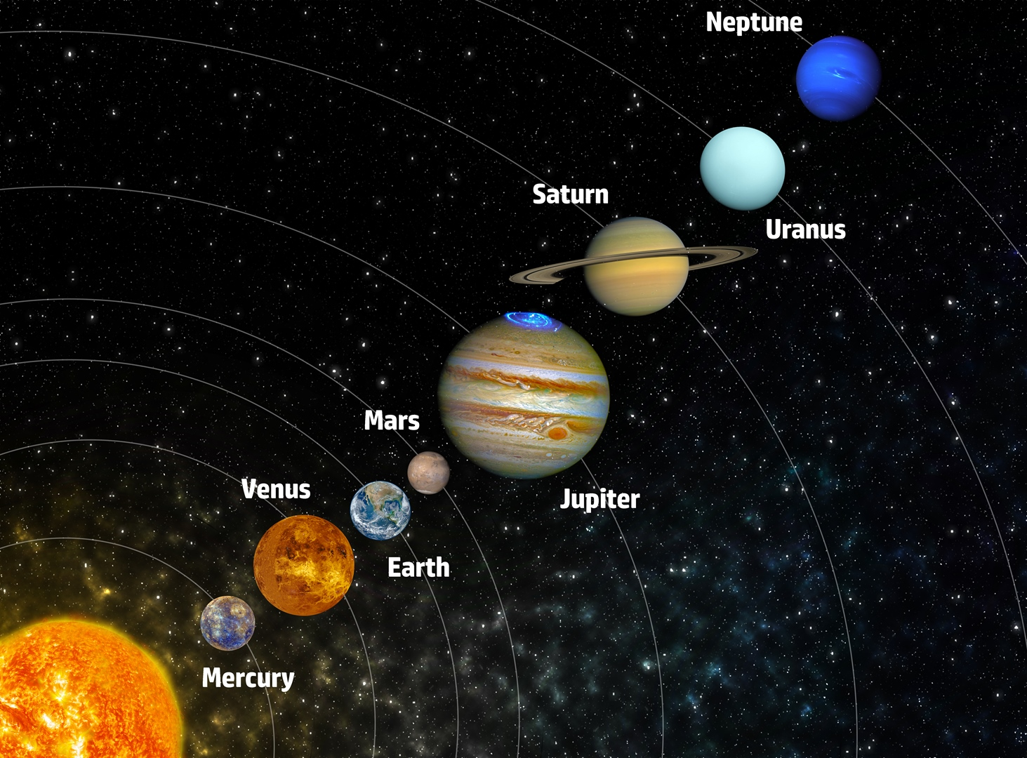
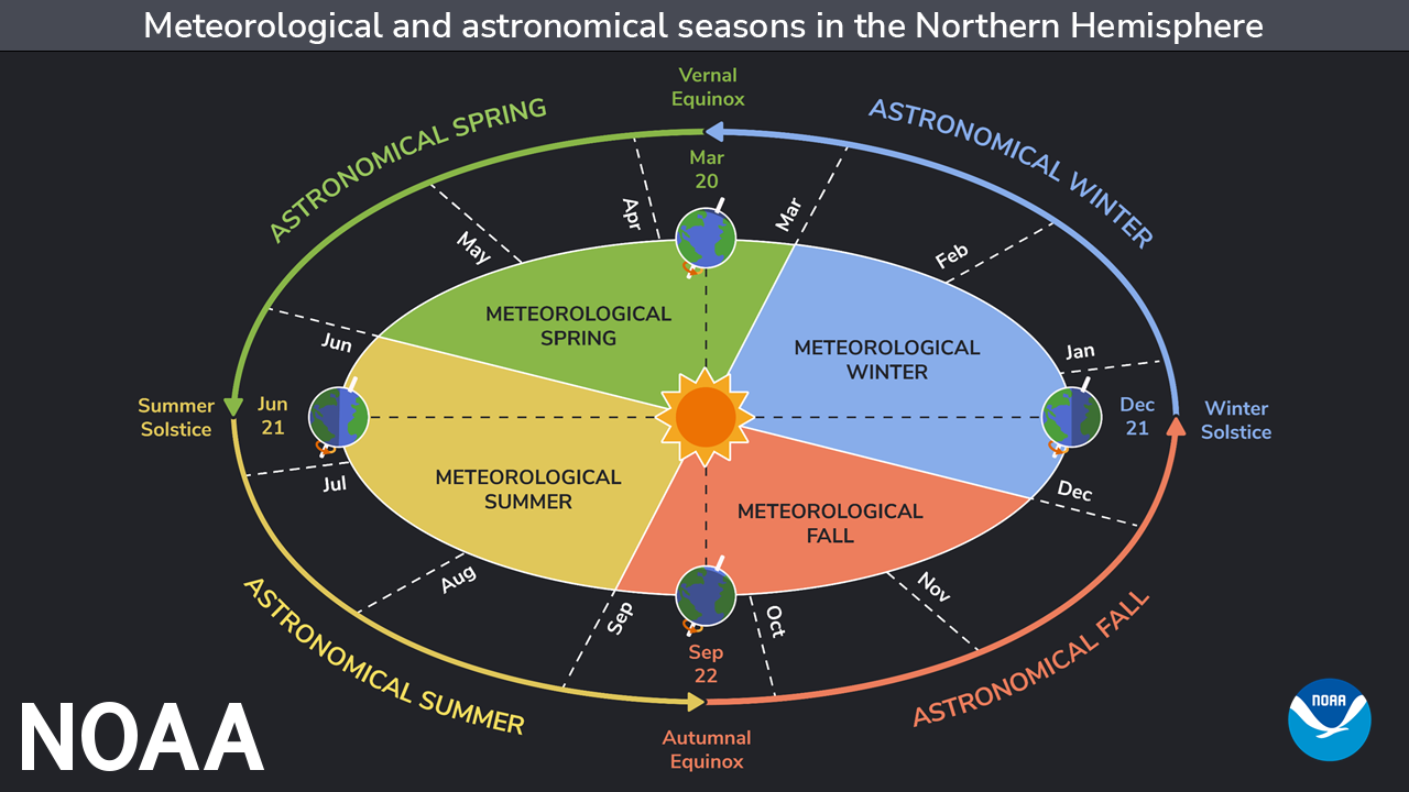
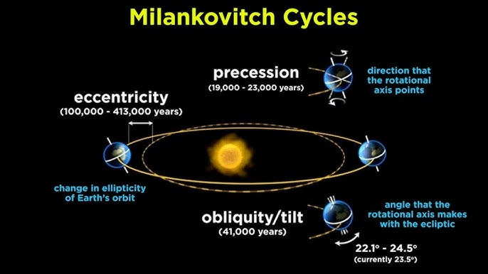
Astronomical processes: Earth’s rotation and orbital translation around the Sun set diurnal and seasonal cycles, modulating the receipt of solar energy.
Atmospheric composition: the proportion of gases such as nitrogen, oxygen, carbon dioxide and water vapour varies in space and time, altering radiative balance and chemical reactions.
Existing temperature and salinity gradients: vertical and horizontal differences in temperature and salinity drive circulation in the oceans and atmosphere.
Processes range from small‑scale turbulence to large‑scale modes of variability such as El Niño–Southern Oscillation, and from slow geological changes to rapid human‑induced alterations.
Climate science therefore tackles questions about natural variability and forced changes, exploring how physical processes and feedbacks give rise to the patterns we observe and how these patterns might evolve. It seeks not only to describe the current climate but also to understand its sensitivity to various drivers, its predictability on different timescales, and its impacts on ecosystems and societies.
Water in the atmosphere can exist as gas, liquid or ice, and transitions between these phases are governed by the triple point conditions of temperature and pressure.
Because the phase diagram of water is tightly constrained by the ambient environment, small changes in energy can shift the balance between vapour, liquid and ice, profoundly affecting clouds and precipitation. Understanding how water absorbs, releases and transports energy is therefore central to climatology.
import numpy as np
import plotly.graph_objects as go
# — Constants
R_u = 8.314462618 # J/(mol·K), universal gas constant
T_trip = 273.16 # K, triple-point temperature
P_trip = 611.657 # Pa, triple-point pressure
# Melting (solid → liquid) at 0 °C
# ΔH_fus = 333.55 kJ/kg × 0.01801528 kg/mol ≈ 6006 J/mol
H_melt = 6006 # J/mol
# Volume change on melting at 0 °C: –1.639 cm³/mol = –1.639e–6 m³/mol
V_melt = -1.639e-6 # m³/mol
# Vaporization (liquid → gas) at 100 °C
# ΔH_vap(100 °C) ≈ 40.657 kJ/mol
H_vap = 40657 # J/mol
T_boil = 373.15 # K, boiling-point temperature at 1 atm
P_boil = 101325 # Pa, standard 1 atm
# Sublimation (solid → gas) at triple point:
# ΔH_sub ≈ ΔH_fus + ΔH_vap(0 °C) ≈ 6006 + (2.5e6 J/kg × 0.01801528 kg/mol) ≈ 51060 J/mol
H_sub = 6006 + (2.5e6 * 0.01801528) # ≈51060 J/mol
# Critical point
T_crit = 647.096 # K
P_crit = 22.064e6 # Pa
# — Temperature arrays
T_melt_arr = np.linspace(T_trip - 5, T_trip, 500) # melting curve
T_vap1_arr = np.linspace(T_trip, T_boil, 500) # liquid→vap (0–1 atm)
T_vap2_arr = np.linspace(T_boil - 50, T_crit, 500) # liquid→vap (1 atm–critical)
T_sub_arr = np.linspace(T_trip - 50, T_trip, 500) # sublimation curve
# — Compute pressures
P_melt_arr = P_trip + (H_melt / V_melt) * np.log(T_melt_arr / T_trip)
P_vap1_arr = P_trip * np.exp((H_vap / R_u) * (1/T_trip - 1/T_vap1_arr))
P_vap2_arr = P_boil * np.exp((H_vap / R_u) * (1/T_boil - 1/T_vap2_arr))
P_sub_arr = P_trip * np.exp((H_sub / R_u) * (1/T_trip - 1/T_sub_arr))
# — Build figure
fig = go.Figure([
go.Scatter(x=T_sub_arr, y=P_sub_arr, mode='lines',
name='Sublimation', line=dict(color='green', width=4)),
go.Scatter(x=T_melt_arr, y=P_melt_arr, mode='lines',
name='Fusion', line=dict(color='black', width=4)),
go.Scatter(x=T_vap1_arr, y=P_vap1_arr, mode='lines',
name='Vapour (0–1 atm)',
line=dict(color='blue', width=4, dash='dash')),
go.Scatter(x=T_vap2_arr, y=P_vap2_arr, mode='lines',
name='Vapour (1 atm–crit)',
line=dict(color='blue', width=4)),
go.Scatter(x=[T_trip], y=[P_trip], mode='markers+text', name='Triple Point',
marker=dict(size=12, color='black'),
text=['Triple Point'], textposition='bottom right'),
go.Scatter(x=[T_crit], y=[P_crit], mode='markers+text', name='Critical Point',
marker=dict(size=12, symbol='diamond', color='black'),
text=['Critical Point'], textposition='top left'),
])
fig.update_layout(
title='Water Phase Diagram (Clausius–Clapeyron)',
xaxis=dict(title='Temperature (K)', range=[200, 700]),
yaxis=dict(title='Pressure (Pa)', type='log'),
width=800,
height=600,
legend=dict(y=0.5),
template='plotly_white'
)
fig.show()
Lecture 1: Atmospheric Composition & Vertical Structure#
1.1 Atmospheric Composition and Mean Molecular Weight#
While people had early ideas about the nature of air, it wasn’t until the late 18th century that scientists began systematically identifying its main components.
Nitrogen (1770s): Daniel Rutherford is credited with the discovery of nitrogen, marking one of the first major steps in understanding air’s composition.
Oxygen (~1770s): Around the same time, Joseph Priestley and Carl Wilhelm Scheele independently discovered oxygen. They originally referred to it as “dephlogisticated air”—a name based on the then-popular (but now obsolete) phlogiston theory.
Once nitrogen and oxygen were recognized as the dominant constituents of the atmosphere, scientists realized that air is composed of roughly:
78% Nitrogen
21% Oxygen
Throughout the late 1700s and early 1800s, this understanding became more refined. Scientists like John Dalton contributed further by identifying and quantifying trace gases such as:
Argon
Carbon dioxide (CO₂)
Ozone (O₃)
Water vapor (H₂O)
Although present in small quantities, these trace constituents (especially H₂O, CO₂ and O₃) play an outsized role in radiative and chemical processes.
In summary, dry air is a mixture, by volume, of
\[ X_{N_2} \approx 0.7808,\quad X_{O_2} \approx 0.2095,\quad X_{Ar} \approx 0.0093,\quad \text{(plus ~0–4% H₂O by volume).} \]Vertical distribution: pressure, temperature and humidity all vary with altitude, defining layers such as the troposphere, stratosphere, mesosphere, etc.
Horizontal distribution: composition and temperature also vary across latitudes, land vs. ocean, and between hemispheres.
Universal gas constant:
\[ R_u = 8.314462618\,\mathrm{J\,mol^{-1}K^{-1}} \]Mean molecular weight of dry air:
\[ M_d = \sum_i X_i\,M_i = 0.7808\,(28.0134) + 0.2095\,(31.9988) + 0.0093\,(39.948) \approx 28.9647\,\mathrm{g/mol} \]Dry-air gas constant:
\[ R_d = \frac{R_u}{M_d/1000} \approx \frac{8.314}{0.0289647} \approx 287.05\,\mathrm{J\,kg^{-1}K^{-1}} \]
1.2. Ideal‐Gas Law for a Mixture#
A gas is considered ideal when it behaves according to the ideal gas law. For a mixture of \(n\) moles of ideal gas at pressure \(p\), volume \(V\) and temperature \(T\):
where \(R_u\) is the universal gas constant. This law assumes that:
Gas molecules occupy no volume.
There are no intermolecular forces between the molecules.
A gas behaves ideally under the following conditions:
Relatively low pressure: Molecules are far apart and do not interact significantly.
Relatively high temperature: Molecules have enough kinetic energy to overcome attractive forces.
Under these circumstances, the assumptions of the ideal gas law are reasonably valid. The gas particles are essentially free to move independently, making the law a good approximation.
At standard temperature and pressure (STP), air behaves very much like an ideal gas. That makes the ideal gas law useful for many practical atmospheric and thermodynamic calculations.
Deviations from Ideal Behavior#
Pressure increases significantly, or
Temperature decreases greatly,
In those cases the molecules are forced closer together, and intermolecular forces and molecular volume can no longer be neglected. In those cases, it is required to account for real gas effects using more advanced models like the van der Waals equation.
If the total mass of gas is \(m\) and the mean molar mass is \(M\), then \(n = m/M\), so:
where
\(R_u = 8.314 \, \text{J/mol·K}\) is the universal gas constant,
\(R = R_u/M\) is the gas constant for the mixture
(e.g.\ \(R_d \approx 287\ \mathrm{J\,kg^{-1}K^{-1}}\) for dry air).\(M\) is the molar mass of the gas (in kg/mol).
Therefore, in mass form:
where:
\(P\) is the pressure of the gas (in Pascals, Pa),
\(\rho\) is the density of the gas (in \(\text{kg/m}^3\)),
\(R\) is the specific gas constant (in J/kg·K),
\(T\) is the absolute temperature of the gas (in Kelvin, K).
This form of the Ideal Gas Law relates the pressure of a gas to its density rather than the amount of gas in moles (\(n\)).
import numpy as np
import plotly.graph_objects as go
from plotly.offline import init_notebook_mode
# Initialize Plotly for Jupyter
init_notebook_mode(connected=True)
# Define ranges for density (ρ) in kg/m³ and temperature (T) in K
rho = np.linspace(0.1, 10, 50) # air density from 0.1 to 10 kg/m³
T = np.linspace(200, 350, 50) # temperature from 200K to 350K
rho, T = np.meshgrid(rho, T)
# Specific gas constant for dry air [J/(kg·K)]
R_specific = 287.05
# Ideal gas law: P = ρ R T
P = rho * R_specific * T # [Pa]
# Plot: Pressure as a function of density and temperature
fig = go.Figure(data=[go.Surface(z=P, x=rho, y=T, colorscale="Viridis")])
# Update layout with correct labels and units
fig.update_layout(
title="Ideal Gas Law (Air): Pressure as a Function of Density and Temperature",
scene=dict(
xaxis_title="Density (ρ) [kg/m³]",
yaxis_title="Temperature (T) [K]",
zaxis_title="Pressure (P) [Pa]",
camera=dict(eye=dict(x=1.2, y=1.2, z=0.8))
),
coloraxis_colorbar=dict(
title="Pressure [Pa]",
titleside="right"
)
)
fig.show()
import numpy as np
import plotly.graph_objects as go
from plotly.offline import init_notebook_mode
# Initialize Plotly for Jupyter
init_notebook_mode(connected=True)
# Define ranges for volume (V) in m³ and temperature (T) in K
V = np.linspace(0.01, 0.2, 50) # volume from 0.001 to 0.1 m³
T = np.linspace(200, 700, 50) # temperature from 200K to 700K
V, T = np.meshgrid(V, T)
# Universal gas constant [J/(mol·K)]
R = 8.314
# Number of moles
n = 1
# Ideal gas law: P = nRT / V
P = (n * R * T) / V # [Pa]
# Plot: Pressure as a function of volume and temperature
fig = go.Figure(data=[go.Surface(z=P, x=V, y=T, colorscale="Cividis")])
# Update layout with correct labels and units
fig.update_layout(
title="Ideal Gas Law: Pressure as a Function of Volume and Temperature",
scene=dict(
xaxis_title="Volume (V) [m³]",
yaxis_title="Temperature (T) [K]",
zaxis_title="Pressure (P) [Pa]",
camera=dict(eye=dict(x=1.4, y=1.2, z=0.9))
),
coloraxis_colorbar=dict(
title="Pressure [Pa]",
titleside="right"
)
)
fig.show()
Dalton’s Law of Partial Pressures#
In a mixture of ideal gases, the total pressure equals the sum of each gas’s partial pressure:
Each component obeys its own ideal‐gas relation:
where
\(m_i\) is the mass of species \(i\),
\(R_i = R_u/M_i\) is its specific gas constant, and
\(\rho_i = m_i/V\) is its partial density.
Because \(V = \sum_i V_i\), one can also define partial volume \(V_i\) by:
Note
The Historical Development of the Ideal Gas Law
The ideal gas law wasn’t discovered all at once—it evolved gradually through the work of several pioneering scientists who uncovered individual relationships between pressure, volume, and temperature.
Key Contributions
Boyle’s Law (1662)
Robert Boyle discovered that the pressure of a gas is inversely proportional to its volume when the temperature is held constant:\[ PV = \text{constant} \quad (T = \text{constant}) \]Charles’s Law (1787)
Jacques Charles found that the volume of a gas is directly proportional to its absolute temperature when the pressure is constant:\[ \frac{V}{T} = \text{constant} \quad (P = \text{constant}) \]Gay-Lussac’s Law (early 1800s)
Joseph Louis Gay-Lussac showed that the pressure of a gas is directly proportional to its absolute temperature when the volume is constant:\[ \frac{P}{T} = \text{constant} \quad (V = \text{constant}) \]
These laws were eventually unified into the ideal gas law.
Theoretical Foundation
Later, the kinetic theory of gases provided a theoretical basis for the ideal gas law. It explained that the observed relationships arise from the motion of gas molecules, assuming:
Molecules move randomly and independently,
Collisions are elastic,
Intermolecular forces are negligible,
Molecules have negligible volume.
This foundation helped solidify the ideal gas law as a cornerstone of thermodynamics and atmospheric science.
1.4 Hydrostatic Balance#
Vertical force balance in a stationary atmosphere:
\[ dp = -\rho\,g\,dz \]Ideal-gas law for dry air:
\[ p = \rho\,R_d\,T \quad \Rightarrow \quad \rho = \frac{p}{R_d\,T} \]Substitute into hydrostatic balance:
\[ \frac{dp}{dz} = -\frac{p}{R_d\,T}\,g \quad \Rightarrow \quad \frac{dp}{p} = -\frac{g}{R_d\,T}\,dz \]Isothermal layer (\(T = \text{const}\)):
\[ \int_{p_0}^{p(z)} \frac{dp}{p} = -\frac{g}{R_d\,T} \int_0^z dz \quad \Rightarrow \quad p(z) = p_0\,\exp\left(-\frac{z}{H}\right) \]Scale height:
\[ H = \frac{R_d\,T}{g} \approx \frac{287\,T}{9.81} \ \mathrm{m} \]
1.3 Density Profile#
From ideal gas:
\[ \rho(z) = \frac{p(z)}{R_d\,T} = \rho_0\,e^{-z/H} \]Examples:
Tropics (\(T \approx 300\) K): \(H \approx 8.78\) km
Poles (\(T \approx 250\) K): \(H \approx 7.30\) km
Lecture 2: Thermodynamic Processes & Lapse Rates#
2.1 First Law of Thermodynamics for a Parcel#
First law per unit mass:
\[ dQ = c_p\,dT - \alpha\,dp, \quad \alpha = \frac{1}{\rho} \]
Lecture 3: Potential Temperature, Static Stability & Brunt–Väisälä#
3.1 Potential Temperature \(\theta\)#
Defined as:
\[ \theta = T\,\left(\frac{p_0}{p}\right)^{R_d/c_p} \]In dry adiabatic motion (\(dQ=0\)), \(\theta\) is conserved:
\[ d\ln \theta = 0 \]
3.2 Static Stability and Brunt–Väisälä Frequency#
Defined as:
\[ N^2 = \frac{g}{\theta}\,\frac{d\theta}{dz} \]Interpretation:
\(N^2 > 0\): stable (parcel oscillates)
\(N^2 < 0\): unstable (parcel rises or sinks)
Typical values:
Tropical troposphere: \(N \sim 0.01\)–0.02 s⁻¹
Stratosphere: \(N \sim 0.02\)–0.05 s⁻¹
Radiative Processes & Energy Balance
Influence on radiative fluxes: gas absorption and emission bands (e.g., H₂O in the infrared, O₃ in the UV) determine how solar and terrestrial radiation is processed.
Energy balance: understanding how incoming solar energy is absorbed, scattered or transmitted, and how outgoing longwave radiation depends on greenhouse gases, is central to climate theory.
Radiative–Convective Equilibrium
In the tropics, the vertical temperature profile often reflects a balance between convective processes (e.g., moist adiabatic ascent) and radiative cooling (primarily via outgoing longwave radiation). This leads to a nearly moist-adiabatic lapse rate with strong control by deep convection.