Stability Index: With spatial calculations#
Bulk Brunt–Väisälä Frequency (N²) Approximation#
The code is computing the Brunt–Väisälä frequency squared using a finite-difference form:
\[
N^2 = \frac{g}{\bar\theta}\,\frac{d\theta}{dz}
\;\;\approx\;\;
\frac{g}{\bar\theta}\,\frac{\theta_{850}-\theta_{1000}}{\Delta z}
\]
Potential Temperature#
Potential temperature at pressure \(p\) is given by Poisson’s equation:
\[
\theta = T \left(\frac{p_0}{p}\right)^\kappa
\]
where
\(T\) is temperature (K),
\(p_0 = 1000\ \text{hPa}\) is the reference pressure,
\(\kappa = R_d / c_p\).
Hypsometric Equation (layer thickness)#
The vertical distance between pressure levels is computed using the dry hypsometric relation with a layer-mean temperature:
\[
\Delta z
= \frac{R_d\,\bar T}{g}\,\ln\!\left(\frac{p_{1000}}{p_{850}}\right)
\]
Final Expression#
Substituting, the bulk \(N^2\) between 1000 and 850 hPa is:
\[
N^2 \;\approx\;
\frac{g}{\tfrac{1}{2}(\theta_{1000}+\theta_{850})}\;
\frac{\theta_{850}-\theta_{1000}}
{\;\dfrac{R_d\,\tfrac{1}{2}(T_{1000}+T_{850})}{g}\,\ln\!\left(\tfrac{p_{1000}}{p_{850}}\right)}
\quad [\text{s}^{-2}]
\]
Assumptions#
Dry air (no virtual temperature correction).
Hydrostatic balance.
Bulk (layer-mean) approximation.
Positive \(N^2\) ⇒ statically stable, negative ⇒ unstable.
import xarray as xr
import numpy as np
import pandas as pd
from pathlib import Path
import xarray as xr
import matplotlib.pyplot as plt
# Resolve path given this notebook lives in intro_to_climatology_repo/data/
candidates = [Path("air.2024.nc"), Path("../data/air.2024.nc"), Path("data/air.2024.nc")]
nc_path = next((p for p in candidates if p.exists()), None)
if nc_path is None:
    raise FileNotFoundError(f"air.2024.nc not found in: {', '.join(map(str, candidates))}")
print("Using:", nc_path)

ds = xr.open_dataset(nc_path, decode_times=True)
print(ds)
Using: data/air.2024.nc
<xarray.Dataset> Size: 262MB
Dimensions:    (level: 17, lat: 73, lon: 144, time: 366, nbnds: 2)
Coordinates:
  * level      (level) float32 68B 1e+03 925.0 850.0 700.0 ... 30.0 20.0 10.0
  * lat        (lat) float32 292B 90.0 87.5 85.0 82.5 ... -85.0 -87.5 -90.0
  * lon        (lon) float32 576B 0.0 2.5 5.0 7.5 ... 350.0 352.5 355.0 357.5
  * time       (time) datetime64[ns] 3kB 2024-01-01 2024-01-02 ... 2024-12-31
Dimensions without coordinates: nbnds
Data variables:
    air        (time, level, lat, lon) float32 262MB ...
    time_bnds  (time, nbnds) float64 6kB ...
Attributes:
    Conventions:    COARDS
    title:          mean daily NMC reanalysis (2014)
    history:        created 2013/12 by Hoop (netCDF2.3)
    description:    Data is from NMC initialized reanalysis\n(4x/day).  It co...
    platform:       Model
    dataset_title:  NCEP-NCAR Reanalysis 1
    References:     http://www.psl.noaa.gov/data/gridded/data.ncep.reanalysis...
# Pick the air temperature variable (or first variable as fallback)
var_name = "air" if "air" in ds.data_vars else list(ds.data_vars)[0]
da = ds[var_name]
print("Variable:", var_name, "| dims:", da.dims, "| units:", da.attrs.get("units", "unknown"))
# Identify coordinate names robustly
lat_name = next((n for n in ["lat", "latitude", "y"] if n in ds.coords), None)
lon_name = next((n for n in ["lon", "longitude", "x"] if n in ds.coords), None)
lev_name = next((n for n in ["level", "lev", "plev", "isobaricInhPa"] if n in ds.coords), None)
print("Coords -> lat:", lat_name, "lon:", lon_name, "lev:", lev_name)
# Quick slice for plotting: first time, and 500 hPa if available
da2 = da.isel(time=0) if "time" in da.dims else da
if lev_name:
try:
# prefer exact 500, else nearest
if 500 in np.array(da2[lev_name]):
da2 = da2.sel({lev_name: 500})
else:
da2 = da2.sel({lev_name: 500}, method="nearest")
except Exception as e:
print("Level selection note:", e)
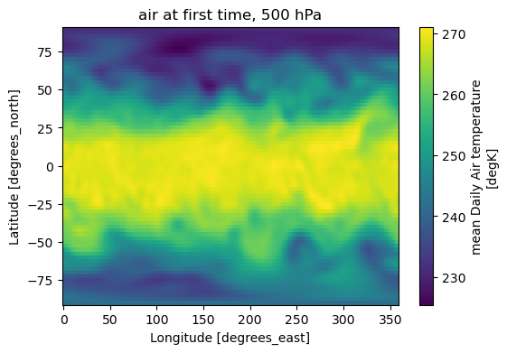
ax = da2.plot(figsize=(6, 4), cmap="viridis")
title = f"{var_name} at first time"
if lev_name:
try:
title += f", {float(da2[lev_name].values):.0f} hPa"
except Exception:
pass
ax.axes.set_title(title)
Variable: air | dims: ('time', 'level', 'lat', 'lon') | units: degK
Coords -> lat: lat lon: lon lev: level
Text(0.5, 1.0, 'air at first time, 500 hPa')
# 3) Select West Pacific point and time
target_lat = 5.0 # degrees North
target_lon = 150.0 # degrees East
# Normalize target lon to dataset's domain
lon_vals = np.asarray(ds[lon_name].values)
if lon_vals.min() >= 0: # dataset uses 0..360
target_lon_ds = target_lon % 360
else: # dataset uses -180..180
target_lon_ds = target_lon if target_lon <= 180 else target_lon - 360
# Choose a time (nearest). Use first time if unsure.
time_sel = ds["time"].values[0]
# Example: pick by date nearest to '2024-07-01'
try:
time_sel = ds["time"].sel(time="2024-07-01", method="nearest").values
except Exception:
pass
# 4) Extract vertical profile at the selected point/time
prof = da.sel({lat_name: target_lat, lon_name: target_lon_ds}, method="nearest").sel(time=time_sel)
# 5) Prepare pressure and temperature
p = prof[lev_name].values # expected in hPa (mb)
T = prof.values # likely in Kelvin; convert to C for readability
units = prof.attrs.get("units", "K")
if units.lower().startswith("k"):
Tplot = T - 273.15
xlab = "Temperature (°C)"
else:
Tplot = T
xlab = f"Temperature ({units})"
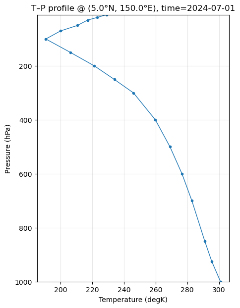
# 6) Plot T vs P
plt.figure(figsize=(5,7))
plt.plot(Tplot, p, marker="o", ms=3, lw=1)
plt.gca().invert_yaxis()
# Optional: set bounds if levels are standard (e.g., 1000→100 hPa)
try:
plt.ylim(max(p), min(p))
except Exception:
pass
plt.xlabel(xlab)
plt.ylabel("Pressure (hPa)")
plt.title(f"T–P profile @ ({target_lat}°N, {target_lon}°E), time={np.datetime_as_string(time_sel, unit='D')}")
plt.grid(True, alpha=0.3)
plt.show()
# ---------------- Config ----------------
target_lat = 5.0     # degN
target_lon = 150.0   # degE
p_bottom = 1000.0    # hPa
p_top = 850.0        # hPa
# ---------------------------------------

# Physical constants
g = 9.80665         # m s^-2
Rd = 287.05         # J kg^-1 K^-1
cp = 1004.0         # J kg^-1 K^-1
kappa = Rd / cp
p0 = 1000.0         # hPa


time_name = "time" if "time" in ds.dims or "time" in ds.coords else None

if any(v is None for v in [lat_name, lon_name, lev_name, time_name]):
    raise ValueError("Could not detect lat/lon/level/time coordinate names.")

# Map longitude to dataset domain
lon_vals = np.asarray(ds[lon_name].values)
if lon_vals.min() >= 0:           # 0..360
    target_lon_ds = target_lon % 360
else:                             # -180..180
    target_lon_ds = target_lon if target_lon <= 180 else target_lon - 360

# Determine pressure unit for interpolation targets
p_coord = ds[lev_name]
p_vals = np.asarray(p_coord.values)
if np.nanmax(p_vals) > 2000:           # Pa
    p_bottom_val = p_bottom * 100.0
    p_top_val = p_top * 100.0
else:                                   # hPa
    p_bottom_val = p_bottom
    p_top_val = p_top

# Extract T(time, level) at the point
prof = da.sel({lat_name: target_lat, lon_name: target_lon_ds}, method="nearest")

# Sort by pressure (ascending) for safe interpolation
prof_sorted = prof.sortby(lev_name)

# Interpolate T at 1000 and 850 hPa for all times (vectorized)
T_bottom = prof_sorted.interp({lev_name: p_bottom_val})
T_top = prof_sorted.interp({lev_name: p_top_val})

# Robust units handling (K, degK, Kelvin, etc.)
units = str(da.attrs.get("units", "K"))
u = units.lower().replace("degrees", "").replace("degree", "").replace("deg", "").replace("°", "").strip()
if u in ("k", "kelvin") or u.endswith("k"):
    pass  # already Kelvin
elif u in ("c", "celsius"):
    T_bottom = T_bottom + 273.15
    T_top = T_top + 273.15
elif u in ("f", "fahrenheit"):
    T_bottom = (T_bottom - 32.0) * 5.0/9.0 + 273.15
    T_top = (T_top - 32.0) * 5.0/9.0 + 273.15
else:
    print(f"Warning: unrecognized temperature units='{units}', assuming Kelvin")

# Potential temperature at endpoints (Poisson eq. expects hPa ratios)
theta_bottom = T_bottom * (p0 / p_bottom) ** kappa
theta_top = T_top * (p0 / p_top) ** kappa
theta_mean = 0.5 * (theta_bottom + theta_top)

# Hypsometric thickness (dry approx; use layer-mean T)
T_mean = 0.5 * (T_bottom + T_top)
dp_ratio = (p_bottom / p_top)  # unitless ratio; same for Pa or hPa
delta_z = (Rd * T_mean / g) * np.log(dp_ratio)   # meters; vector over time

# Bulk N^2 per day over 1000–850 hPa
N2 = (g / theta_mean) * (theta_top - theta_bottom) / delta_z  # s^-2; DataArray over time
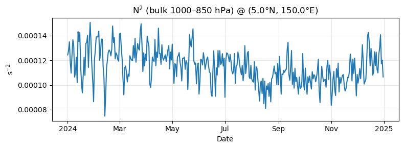
fig, ax = plt.subplots(figsize=(8, 3))
N2.plot(ax=ax, color="tab:blue")
ax.set_title(f"N$^2$ (bulk 1000–850 hPa) @ ({target_lat}°N, {target_lon}°E)")
ax.set_ylabel("s$^{-2}$")
ax.set_xlabel("Date")
ax.grid(True, alpha=0.3)
plt.tight_layout()
# Bulk N^2 (1000–850 hPa) for all pixels in 15S–15N, for all times
from pathlib import Path
import numpy as np
import xarray as xr
import matplotlib.pyplot as plt
# ---------------- Config ----------------
p_bottom = 1000.0 # hPa
p_top = 850.0 # hPa
lat_min, lat_max = -15.0, 15.0
# ---------------------------------------
# Physical constants
g = 9.80665 # m s^-2
Rd = 287.05 # J kg^-1 K^-1
cp = 1004.0 # J kg^-1 K^-1
kappa = Rd / cp
p0 = 1000.0 # hPa
# Open dataset (adjust path if needed)
nc_path = Path("data/air.2024.nc")
if not nc_path.exists():
for p in [Path("air.2024.nc"), Path("../data/air.2024.nc")]:
if p.exists():
nc_path = p
break
print("Using:", nc_path)
ds = xr.open_dataset(nc_path, decode_times=True)
# Identify variable and coordinates
var_name = "air" if "air" in ds.data_vars else list(ds.data_vars)[0]
da = ds[var_name]
lat_name = next((n for n in ["lat", "latitude", "y"] if n in ds.coords), None)
lon_name = next((n for n in ["lon", "longitude", "x"] if n in ds.coords), None)
lev_name = next((n for n in ["level", "lev", "plev", "isobaricInhPa"] if n in ds.coords), None)
time_name = "time" if "time" in ds.dims or "time" in ds.coords else None
if any(v is None for v in [lat_name, lon_name, lev_name, time_name]):
raise ValueError("Could not detect lat/lon/level/time coordinate names.")
# Subset tropical band (robust to ascending/descending latitude order)
lat_vals = ds[lat_name].values
ascending = (lat_vals[-1] - lat_vals[0]) > 0
lat_slice = slice(lat_min, lat_max) if ascending else slice(lat_max, lat_min)
da_trop = da.sel({lat_name: lat_slice})
# Determine pressure units and targets for interpolation
p_coord = ds[lev_name]
p_vals = np.asarray(p_coord.values)
if np.nanmax(p_vals) > 2000: # Pa
p_bottom_val = p_bottom * 100.0
p_top_val = p_top * 100.0
else: # hPa
p_bottom_val = p_bottom
p_top_val = p_top
# Sort by pressure (ascending) and interpolate to 1000/850 hPa across all time/lat/lon
da_sorted = da_trop.sortby(lev_name)
T_bottom = da_sorted.interp({lev_name: p_bottom_val})
T_top = da_sorted.interp({lev_name: p_top_val})
# Robust units handling (K, degK, Kelvin, etc.)
units = str(da.attrs.get("units", "K"))
u = units.lower().replace("degrees", "").replace("degree", "").replace("deg", "").replace("°", "").strip()
if u in ("k", "kelvin") or u.endswith("k"):
pass # already Kelvin
elif u in ("c", "celsius"):
T_bottom = T_bottom + 273.15
T_top = T_top + 273.15
elif u in ("f", "fahrenheit"):
T_bottom = (T_bottom - 32.0) * 5.0/9.0 + 273.15
T_top = (T_top - 32.0) * 5.0/9.0 + 273.15
else:
print(f"Warning: unrecognized temperature units='{units}', assuming Kelvin")
# Mask where interpolation failed (e.g., 1000 hPa below surface)
valid = np.isfinite(T_bottom) & np.isfinite(T_top)
T_bottom = T_bottom.where(valid)
T_top = T_top.where(valid)
# Potential temperature at endpoints (Poisson equation expects hPa ratios)
theta_bottom = T_bottom * (p0 / p_bottom) ** kappa
theta_top = T_top * (p0 / p_top) ** kappa
theta_mean = 0.5 * (theta_bottom + theta_top)
# Hypsometric thickness (dry; use layer-mean T)
T_mean = 0.5 * (T_bottom + T_top)
dp_ratio = (p_bottom / p_top) # unitless
delta_z = (Rd * T_mean / g) * np.log(dp_ratio) # meters
# Bulk N^2 for every time/lat/lon in the tropical band
N2 = (g / theta_mean) * (theta_top - theta_bottom) / delta_z # s^-2
N2 = N2.rename("N2_1000_850").assign_attrs(units="s^-2", long_name="Bulk Brunt–Väisälä frequency squared (1000–850 hPa)")
print(N2)
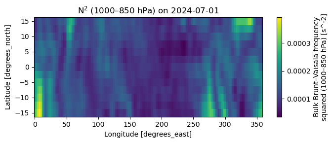
# Example 1: Map for a chosen day (nearest)
day = "2024-07-01"
fig, ax = plt.subplots(figsize=(7,3))
N2.sel({time_name: day}, method="nearest").plot(ax=ax, cmap="viridis")
ax.set_title(f"N$^2$ (1000–850 hPa) on {day}")
plt.tight_layout()
plt.show()
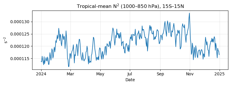
# Example 2: Tropical-mean daily series (average over lat,lon in 15S–15N)
N2_mean = N2.mean(dim=[lat_name, lon_name], skipna=True)
fig, ax = plt.subplots(figsize=(8,3))
N2_mean.plot(ax=ax, color="tab:blue")
ax.set_title("Tropical-mean N$^2$ (1000–850 hPa), 15S–15N")
ax.set_ylabel("s$^{-2}$"); ax.set_xlabel("Date"); ax.grid(True, alpha=0.3)
plt.tight_layout()
plt.show()
Using: data/air.2024.nc
<xarray.DataArray 'N2_1000_850' (time: 366, lat: 13, lon: 144)> Size: 5MB
array([[[1.45438151e-04, 1.74229465e-04, 2.04747667e-04, ...,
         1.56576612e-04, 1.50732930e-04, 1.39069289e-04],
        [1.44379390e-04, 1.82302789e-04, 2.14797760e-04, ...,
         1.34017226e-04, 1.22970268e-04, 1.22950591e-04],
        [1.23578022e-04, 1.46168422e-04, 1.68797188e-04, ...,
         1.13106816e-04, 1.01467539e-04, 1.05571757e-04],
        ...,
        [1.48090198e-04, 1.60636765e-04, 1.79558523e-04, ...,
         1.12719112e-04, 1.22922931e-04, 1.36116130e-04],
        [1.62414941e-04, 1.89293268e-04, 2.28866668e-04, ...,
         1.05044590e-04, 1.28017013e-04, 1.46754594e-04],
        [1.44882018e-04, 1.88802954e-04, 2.60040718e-04, ...,
         8.51524555e-05, 1.08851125e-04, 1.26565076e-04]],

       [[1.93032171e-04, 2.35483560e-04, 2.56884641e-04, ...,
         1.96457484e-04, 1.78224278e-04, 1.70023971e-04],
        [1.73466983e-04, 2.14600135e-04, 2.38956042e-04, ...,
         1.61240652e-04, 1.43902751e-04, 1.44460528e-04],
        [1.41049365e-04, 1.56612612e-04, 1.65298416e-04, ...,
         1.19844420e-04, 1.16379802e-04, 1.25552545e-04],
...
        [2.54333877e-04, 2.48332101e-04, 2.54699332e-04, ...,
         2.67835279e-04, 2.66103332e-04, 2.63801783e-04],
        [2.75898354e-04, 2.87480169e-04, 3.09121722e-04, ...,
         2.81060770e-04, 2.75367529e-04, 2.74287106e-04],
        [2.81197352e-04, 3.03781780e-04, 3.39139546e-04, ...,
         2.72706103e-04, 2.71895765e-04, 2.73859607e-04]],

       [[2.16650559e-04, 2.39262546e-04, 2.58274808e-04, ...,
         2.20734752e-04, 2.14021779e-04, 2.07655722e-04],
        [1.98547133e-04, 2.27596742e-04, 2.52360158e-04, ...,
         2.15625869e-04, 2.00779160e-04, 1.89392617e-04],
        [1.62404569e-04, 1.92590876e-04, 2.23486377e-04, ...,
         1.78212241e-04, 1.65923775e-04, 1.54252462e-04],
        ...,
        [2.86012871e-04, 2.77413639e-04, 2.65786815e-04, ...,
         2.99703891e-04, 2.90567602e-04, 2.89950191e-04],
        [3.16622597e-04, 3.17094998e-04, 3.13155477e-04, ...,
         3.25579091e-04, 3.15570659e-04, 3.13256335e-04],
        [3.16743890e-04, 3.22656385e-04, 3.31828517e-04, ...,
         3.22199999e-04, 3.15539566e-04, 3.15618215e-04]]])
Coordinates:
  * lat      (lat) float32 52B 15.0 12.5 10.0 7.5 5.0 ... -7.5 -10.0 -12.5 -15.0
  * lon      (lon) float32 576B 0.0 2.5 5.0 7.5 10.0 ... 350.0 352.5 355.0 357.5
  * time     (time) datetime64[ns] 3kB 2024-01-01 2024-01-02 ... 2024-12-31
Attributes:
    units:      s^-2
    long_name:  Bulk Brunt–Väisälä frequency squared (1000–850 hPa)
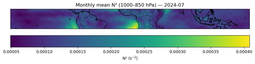
# Monthly N^2 (1000–850 hPa) map with Cartopy
import numpy as np
import xarray as xr
import matplotlib.pyplot as plt
import cartopy.crs as ccrs
import cartopy.feature as cfeature

# Expect a DataArray named N2 with dims like (time, lat, lon)
if "N2" not in globals():
    raise NameError("N2 not found. Compute N2 first (time, lat, lon).")

# Coordinate names (robust detection)
lat_name = next((n for n in ["lat", "latitude", "y"] if n in N2.dims or n in N2.coords), None)
lon_name = next((n for n in ["lon", "longitude", "x"] if n in N2.dims or n in N2.coords), None)
time_name = next((n for n in ["time", "date"] if n in N2.dims or n in N2.coords), None)
if any(v is None for v in [lat_name, lon_name, time_name]):
    raise ValueError("Could not detect lat/lon/time coordinate names on N2.")

# Resample to monthly means
N2_mon = N2.resample({time_name: "MS"}).mean(skipna=True)

# Select a month to plot
month_str = "2024-07"  # change as needed
da_mon = N2_mon.sel({time_name: month_str}, method="nearest")

# Shift longitude to [-180, 180] for nicer world map (optional but recommended)
lon_vals = xr.DataArray(N2[lon_name])
if float(lon_vals.max()) > 180:
    lon_shifted = ((lon_vals + 180) % 360) - 180
    da_mon = da_mon.assign_coords({lon_name: lon_shifted}).sortby(lon_name)

# Plot with Cartopy
fig = plt.figure(figsize=(9, 5))
proj = ccrs.PlateCarree()
ax = plt.axes(projection=proj)

# Focus on tropics; widen a bit for context
ax.set_extent([-180, 180, -15, 15], crs=ccrs.PlateCarree())
ax.coastlines(linewidth=0.8)
ax.add_feature(cfeature.BORDERS, linewidth=0.3)
ax.add_feature(cfeature.LAND, facecolor="0.95", edgecolor="none", zorder=0)

# Use xarray's plot with proper transform
pcm = da_mon.plot(
    ax=ax,
    transform=ccrs.PlateCarree(),
    cmap="viridis",
    add_colorbar=True,
    cbar_kwargs={"label": "N² (s$^{-2}$)", "orientation": "horizontal", "pad": 0.05},
)

# Title
tlabel = np.datetime_as_string(da_mon[time_name].values, unit="M")
ax.set_title(f"Monthly mean N² (1000–850 hPa) — {tlabel}")

plt.tight_layout()
plt.show()